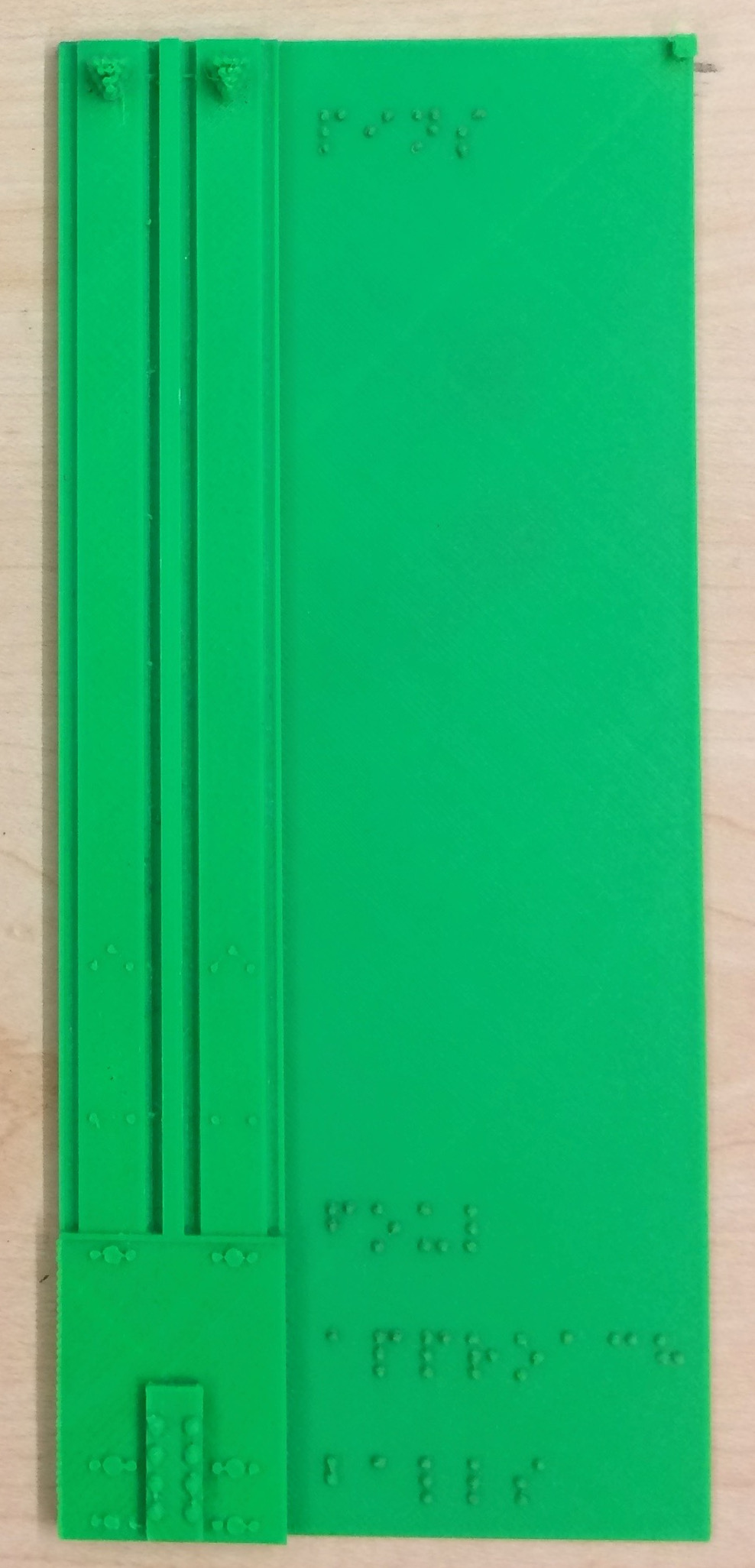
GS 8-dot Braille Slate
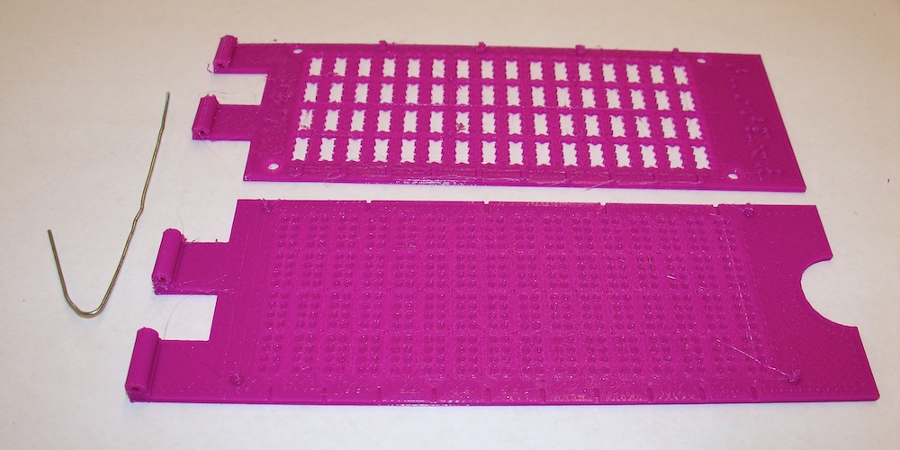
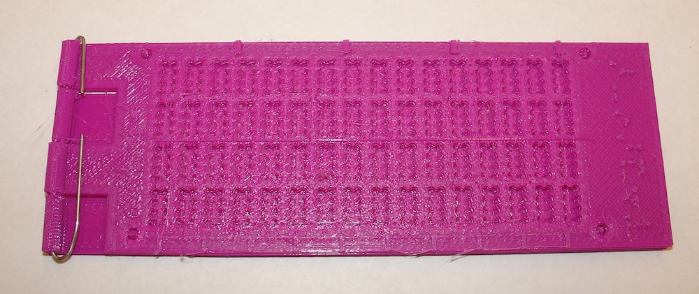
This slate was designed by UW-Whitewater physics student Chris Marshall as part of Spring 2015 student research funding by the UW-Whitewater Provost's office.
This model has been uploaded to YouMagine as: 8-dot Braille Slate
Files to download:
Slate .stl file.
This model will need to be rescaled by a factor of 10x in your 3D program.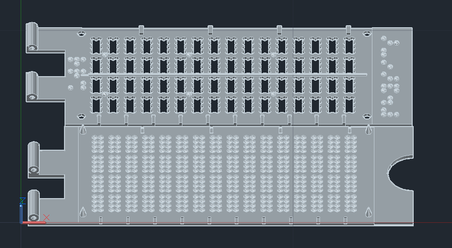 Slate .dwg.zip (zipped AutoCAD file.)
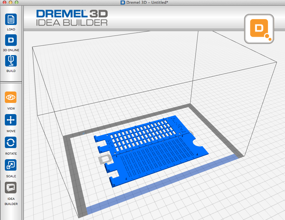 Slate .3dremel.zip (zipped Dremel Idea Builder file.)
Build time is approximately 2.5 hrs.
Information about GS Braille:
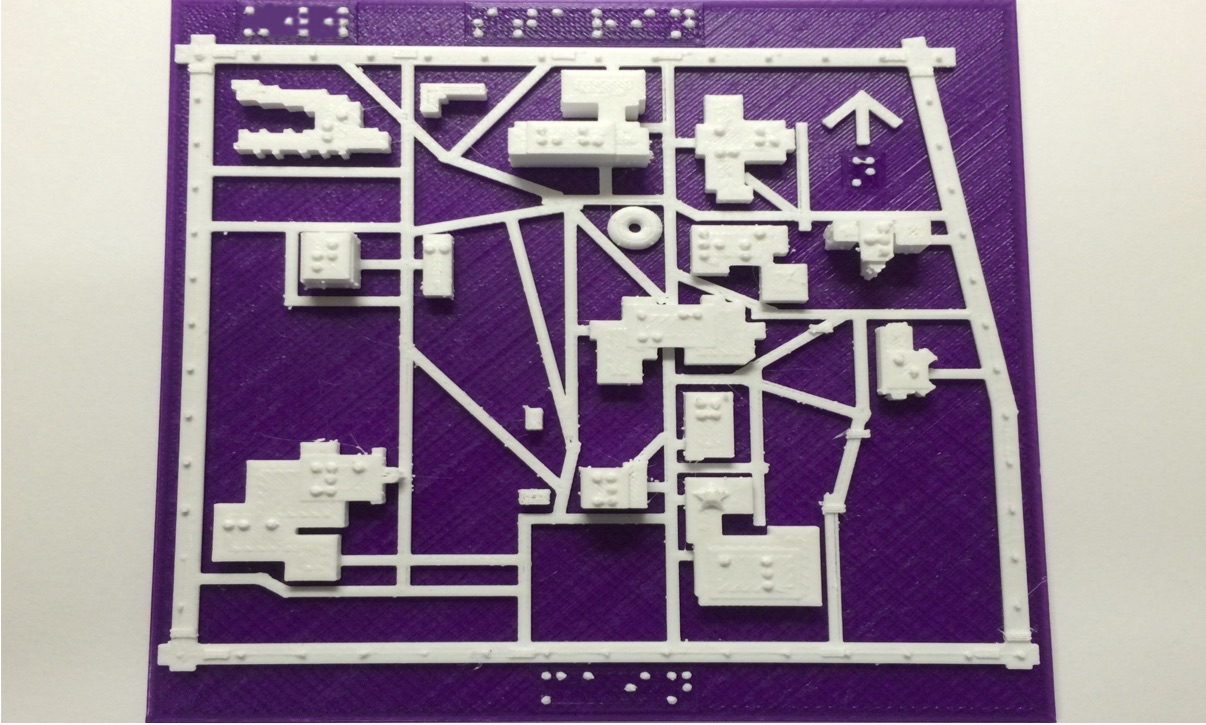
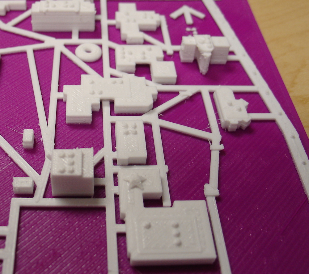
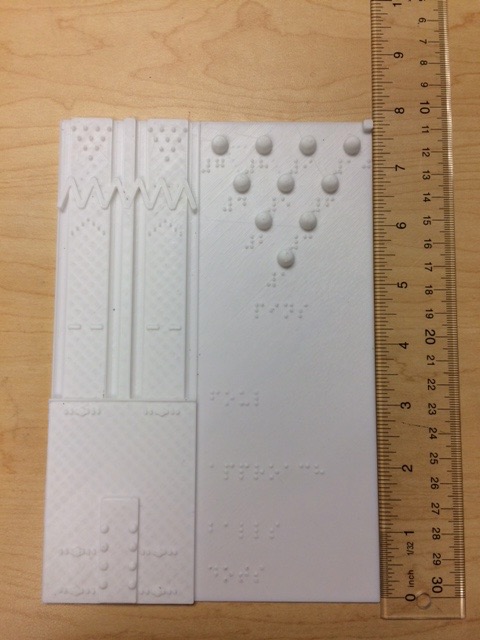
University of Wisconsin - Whitewater 3D Central campus map
For a tactile map of a location of your choice, I
Build time is approximately 4.5 hrs.
This map was designed by Steven Sahyun, 2015
Features and Guide for the UWW campus map:
Files to download:
UWW map .stl file.
This model will need to be reduced to about 1% (0.93%) the original in your 3D program. UWW map .dwg.zip (zipped AutoCAD file.)
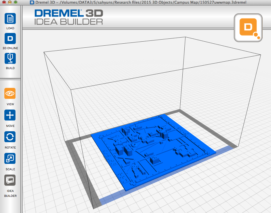 UWW map .3dremel.zip (zipped Dremel Idea Builder file.)
Map labels and touch-cons
Pulley system
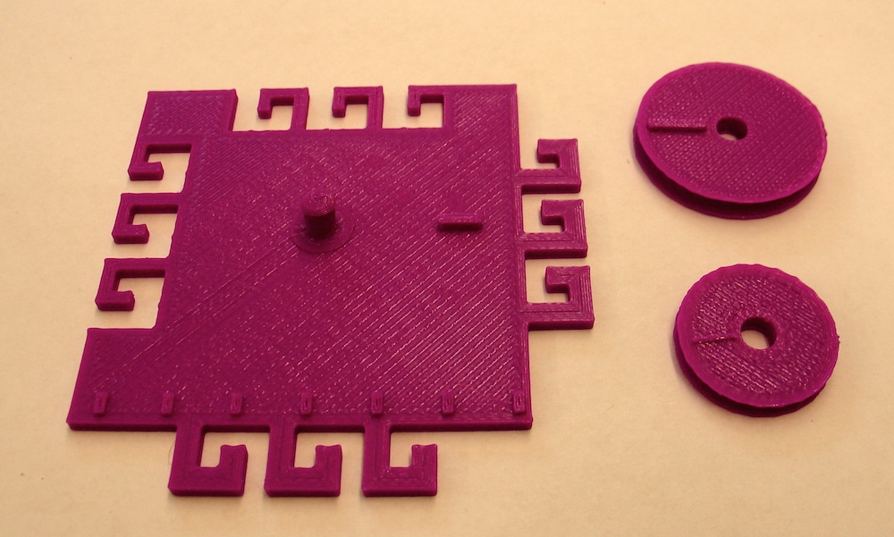
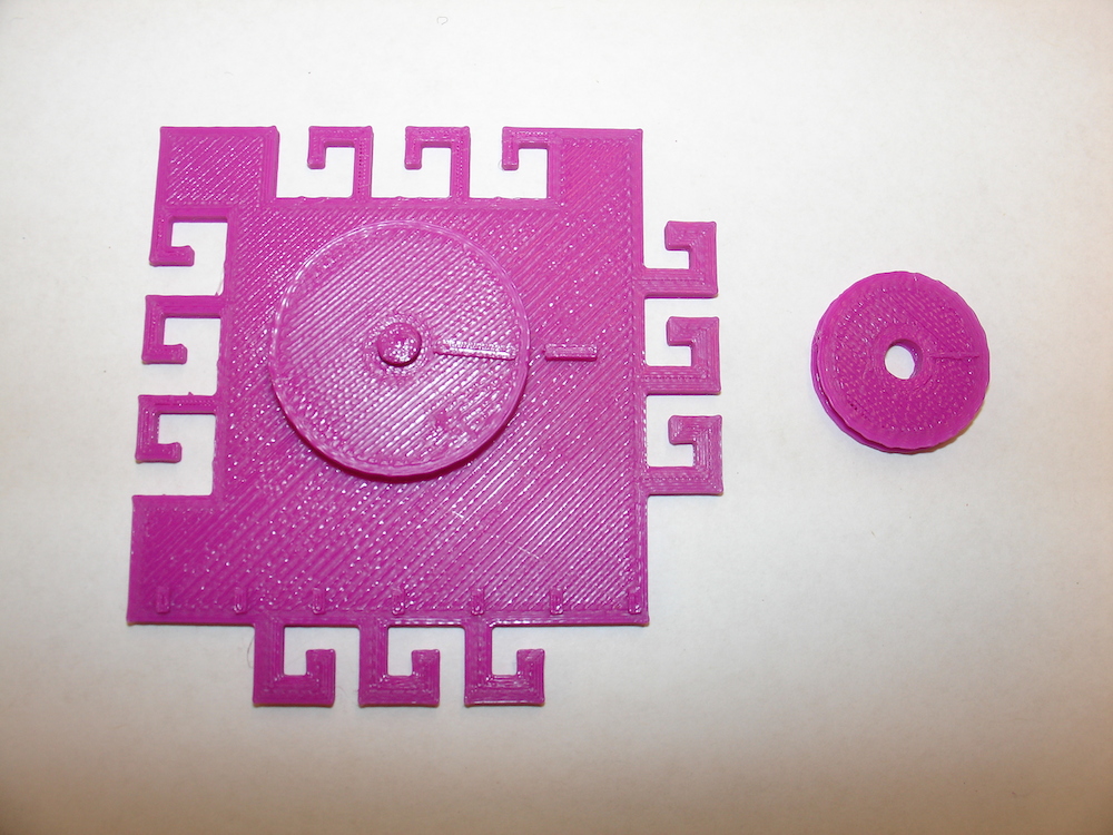
This is a printable pulley system. The file contains two pulleys, a large wheel and a small wheel; the smaller wheel is useful when creating systems with 3 or 4 pulleys.
Files to download:
Pulley .stl file.
This model should be scaled correctly in your 3D program.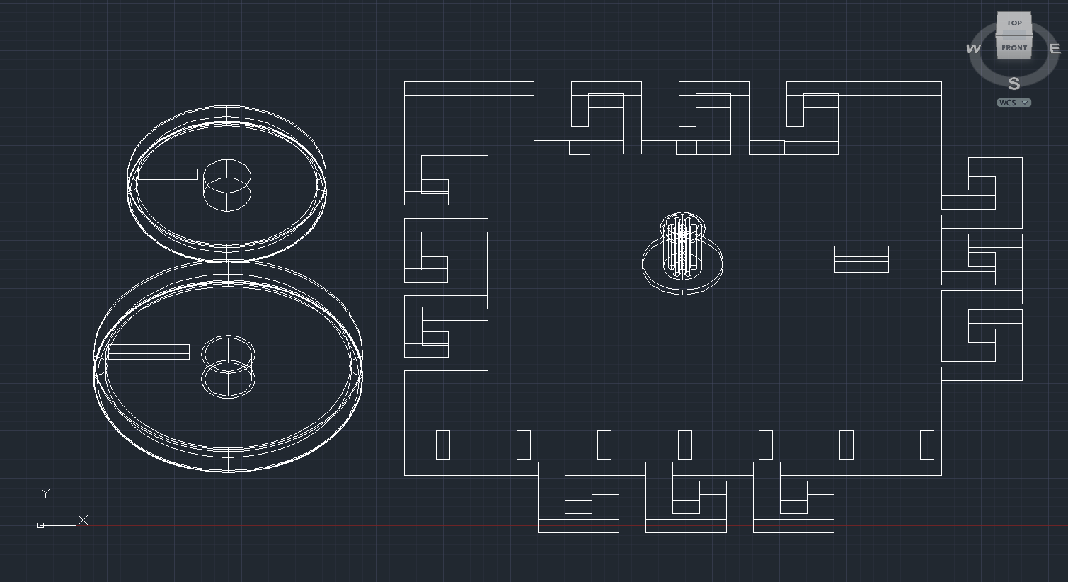 Pulley .dwg.zip (zipped AutoCAD file.)
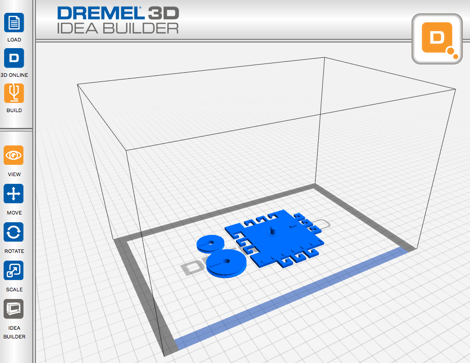 Pulley .3dremel.zip (zipped Dremel Idea Builder file.)
Build time is approximately 45 min.
Features of the pulley system:
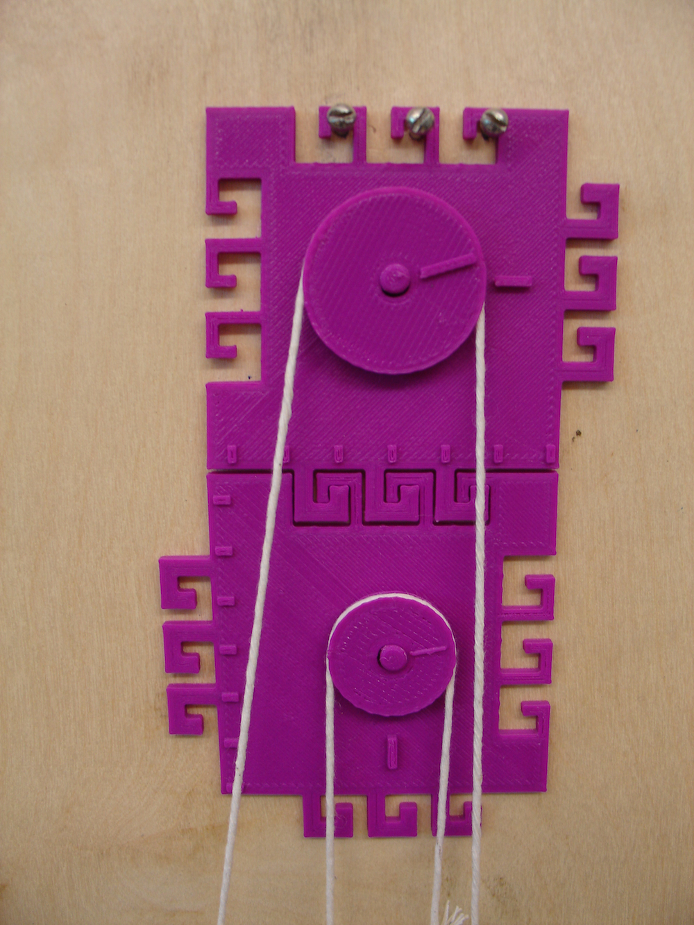
The pulley is designed with tactile indicators on the pulley wheel and on the pulley base so students can feel the rotations of the wheel as the pulley is used. By comparing the rotational rates between a simple and combined pulley systems, students can feel the difference in how much the pulley moves for different configurations. In addition, the pulley base is designed in an interlocking pattern of hooks so that pulleys can be easily linked together.
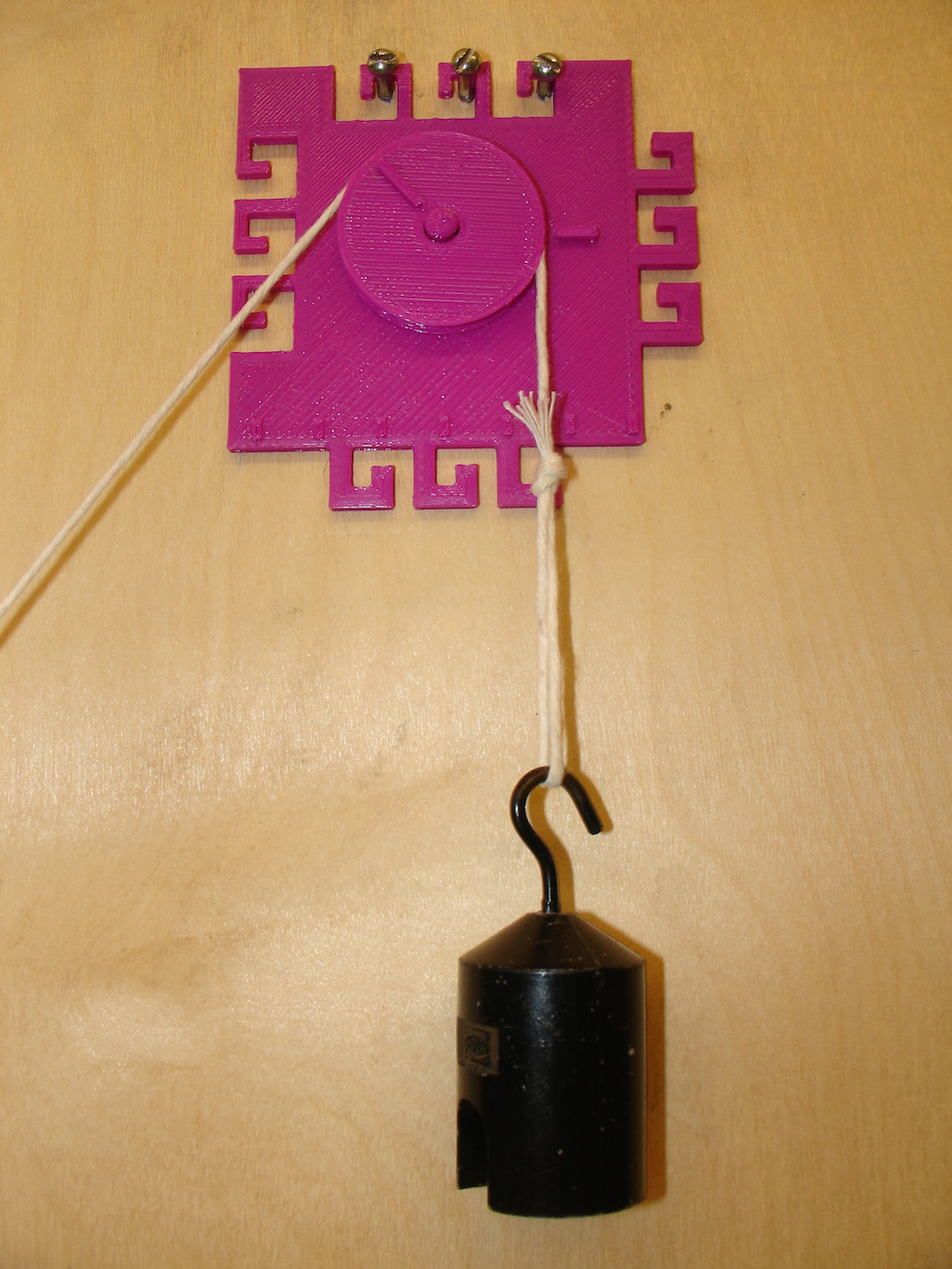
There are two sets of three hooks for the pulley base. This allows greater stability when attaching the pulley to a base-board (It is recommended using three screws in a wood board to hook the pulley base onto. There are two orientations that the base may be attached; the redundancy is useful in the event that one of the hooks breaks.
Single Pulley configuration:
Two Pulley configuration: Note that the string attaches to the upper pulley base hook.
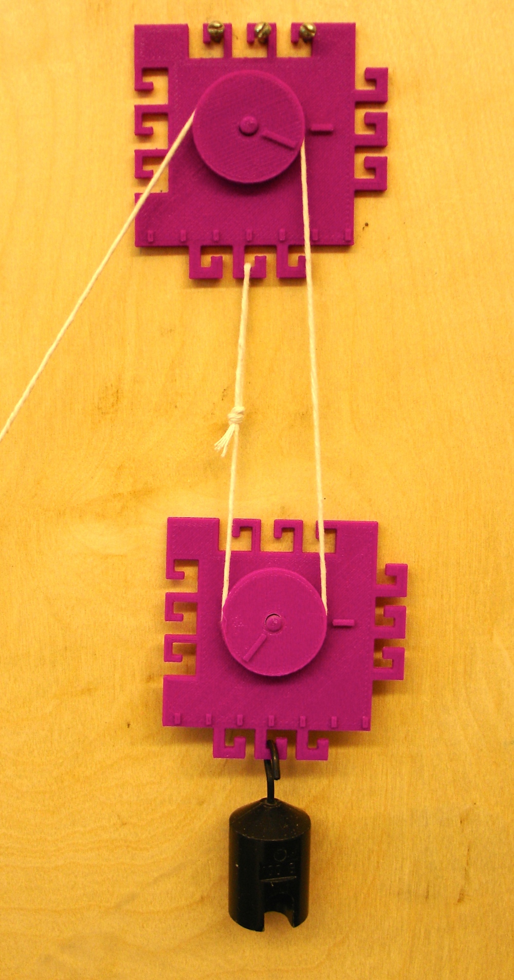
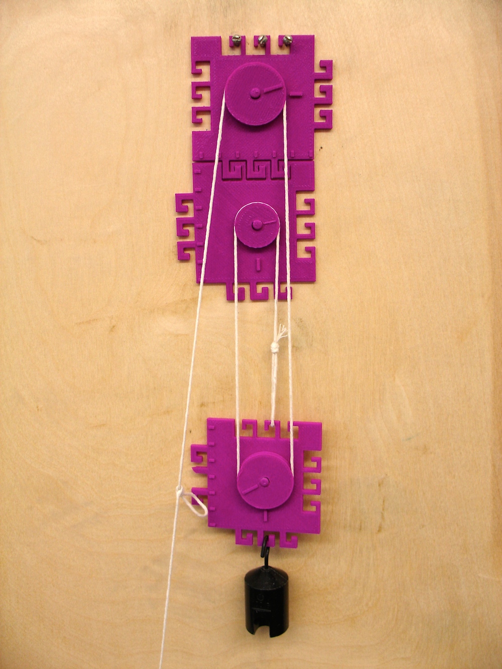
Three Pulley configuration: Note that the string attaches to the lower pulley base hook and that the two upper pulleys lock together.
Useful information about the mechanical advantage for a pulley system can be found at: http://en.wikipedia.org/wiki/Mechanical_advantage_device. The following image shows 1, 2, 3, and 4 pulley systems that this 3D object can replicate.

Image credit: Prolineserver, Tomia, and Stanislaw Skowron from Wikipedia (2015).
This pulley was designed by UW-Whitewater physics student Rebecca Holzer as part of Spring 2015 student research funding by the UW-Whitewater Provost's office. Additional design revisions by Steven Sahyun.
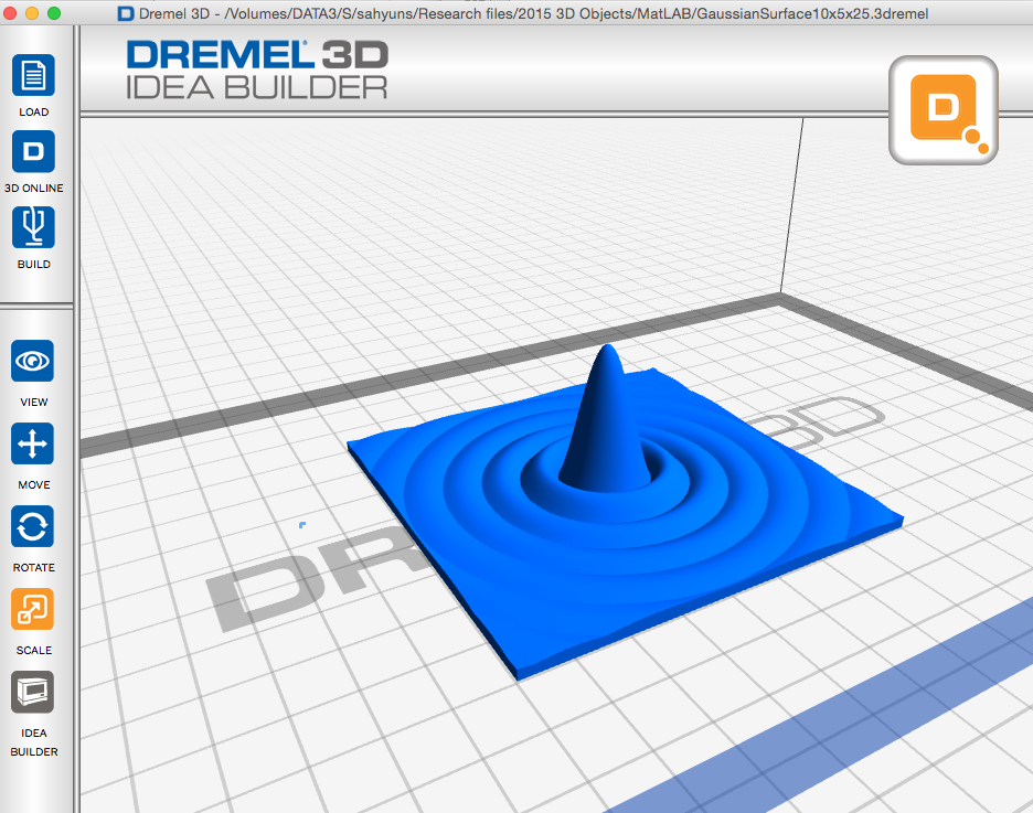
Normal (Gaussian) Distributions
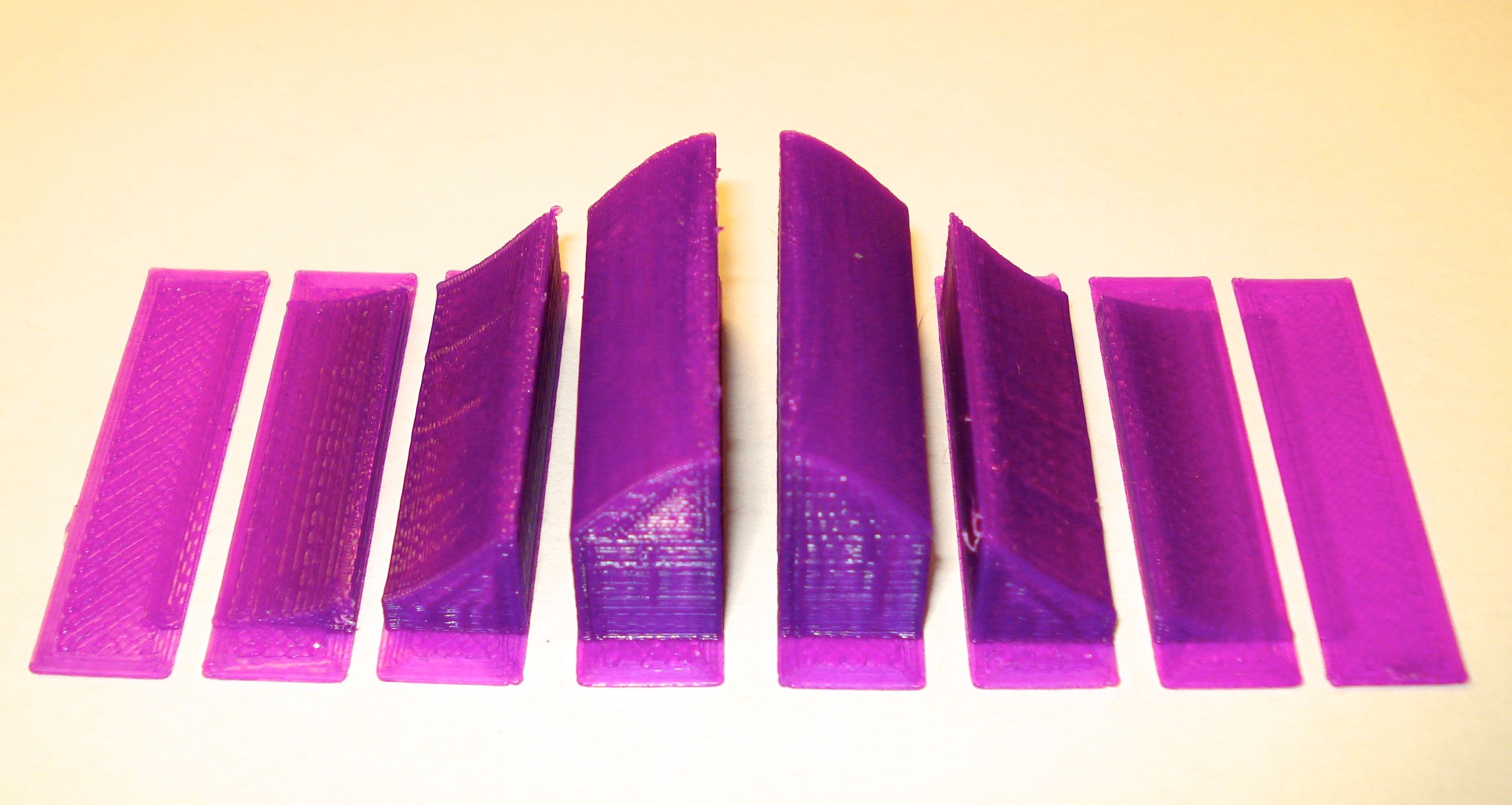
Here is the classic normal (Gaussian) distribution and the distribution separated into one standard deviation (1 σ) segments. These have been calculated using the MatLAB code below.
Files to download:
Set of .stl files
This file contains the entire distribution and the distribution broken down as segments (0-1 σ, 1-2 σ, 2-3 σ and 3-4 σ). This model may be printed at any size.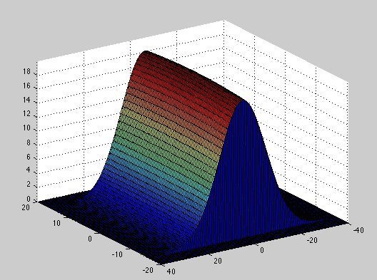 gaussian2d.m MatLAB code
This MatLAB code uses the stlwrite and surf2solid functions by Sven Holcombe. Instructions for exporting stl files from MatLAB.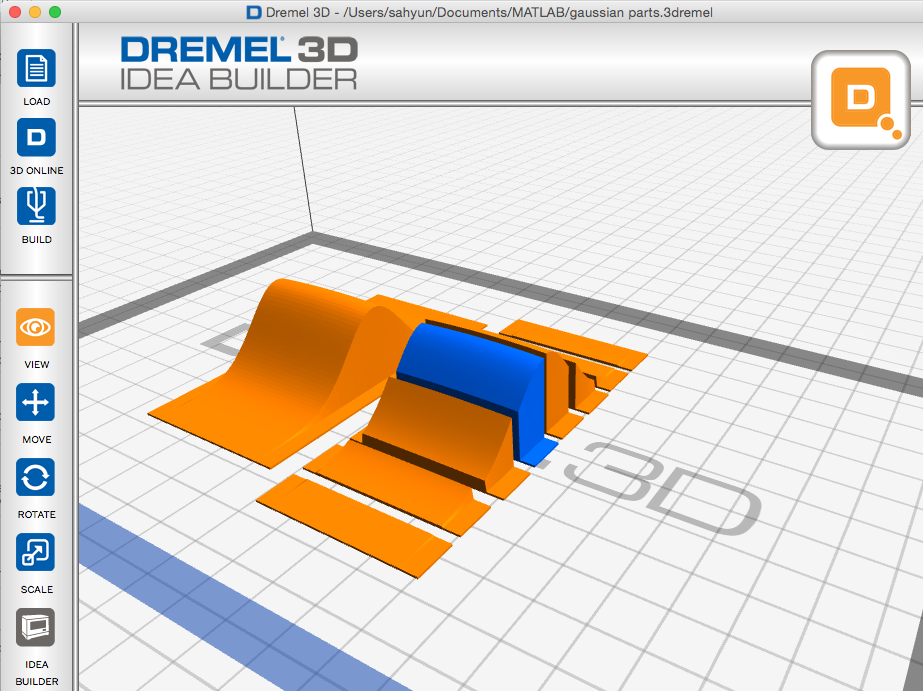 2D Gaussian .3dremel.zip (zipped Dremel Idea Builder file) Consisting of the full distribution and parts from -4 σ to +4 σ scaled to 5 cm by 8 cm
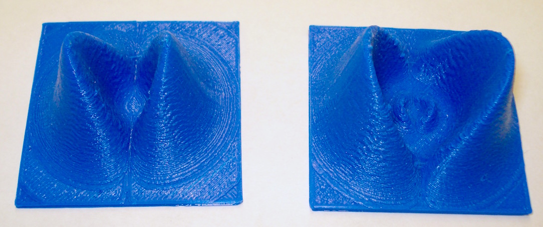
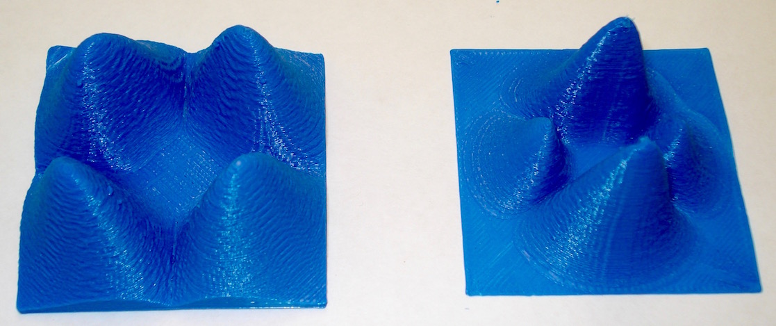
Symmetric and Asymmetric distributions
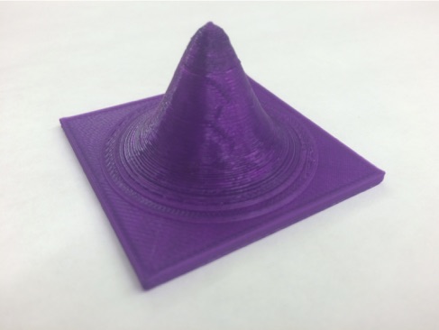
Here are two more normal distribution files that have been calculated using MatLAB. The first is a symmetric distribution (x and y have the same standard deviation.) This is the case for a laser beam or a Bose-Einstein condensate. The second file is an asymmetric distribution (standard deviation of x is different than that for y.) This could be the profile for a diode laser. The asymmetric profile feels more interesting and shows what it means when the standard deviation is different for similar conditions.
Files to download:
Symmetric gaussian .stl file.
This model may be printed at any size.Asymmetric gaussian .stl file.
This model may be printed at any size.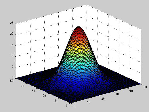 gaussian.m MatLAB code
This MatLAB code uses the stlwrite and surf2solid functions by Sven Holcombe. Instructions for exporting stl files from MatLAB.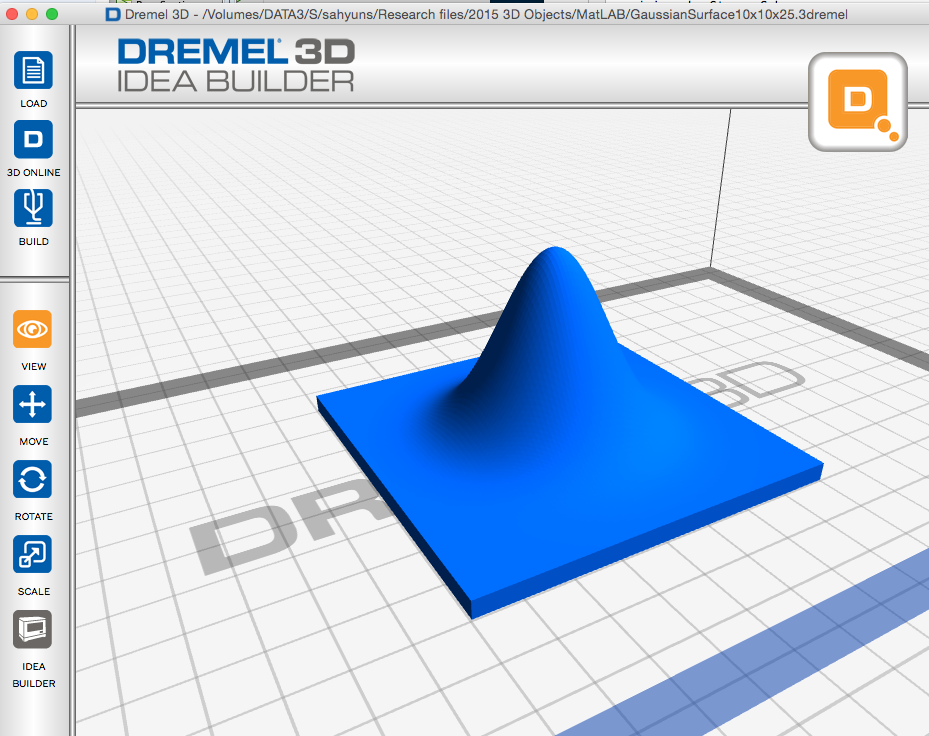 Symmetric gaussian .3dremel.zip (zipped Dremel Idea Builder file) scaled to 8 cm by 8 cm
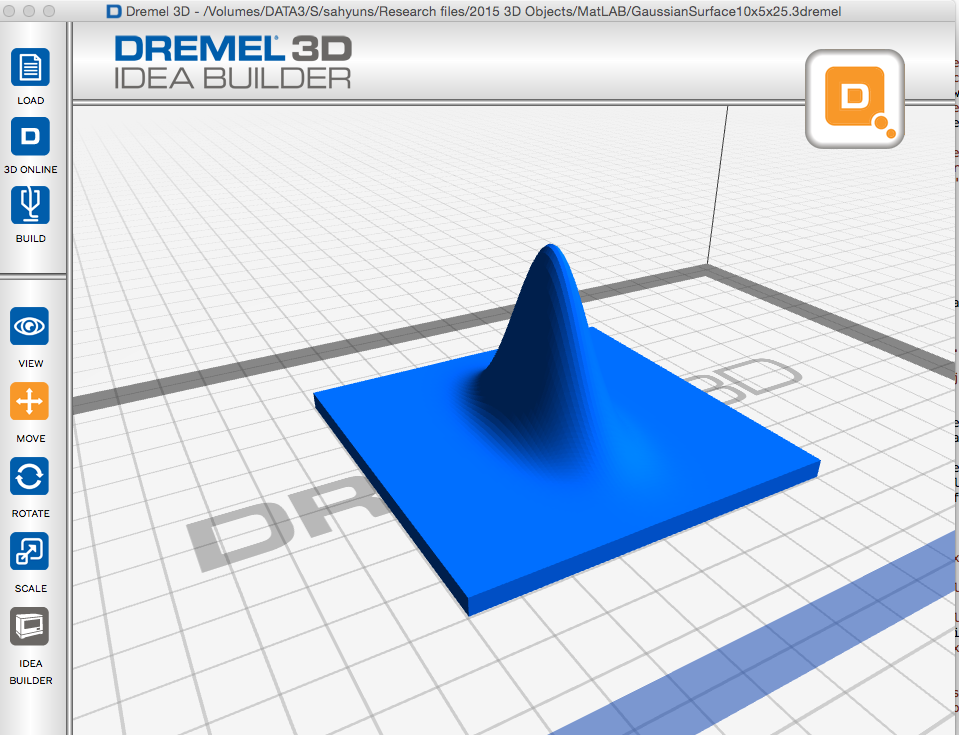 Asymmetric gaussian .3dremel.zip (zipped Dremel Idea Builder file) scaled to 8 cm by 8 cm
Build time for these are approximately 1 hr each.
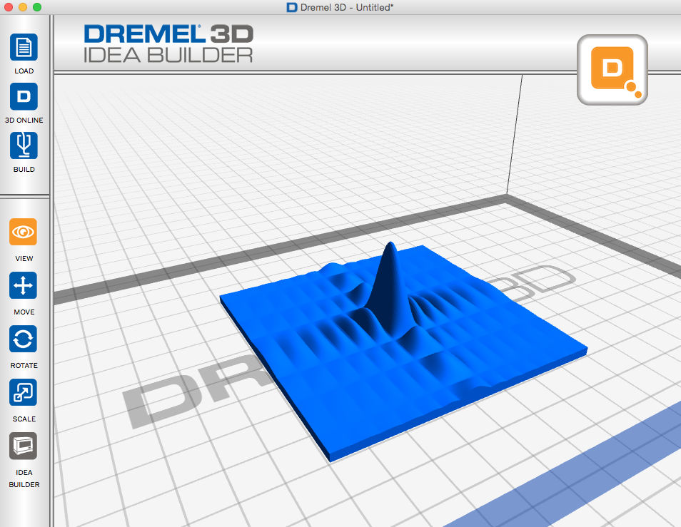
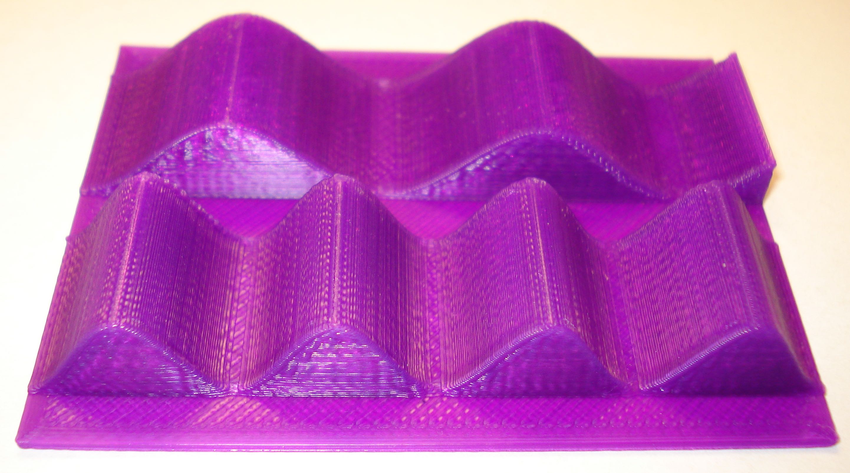
Diffraction Patterns for Circular and Rectangular Apertures
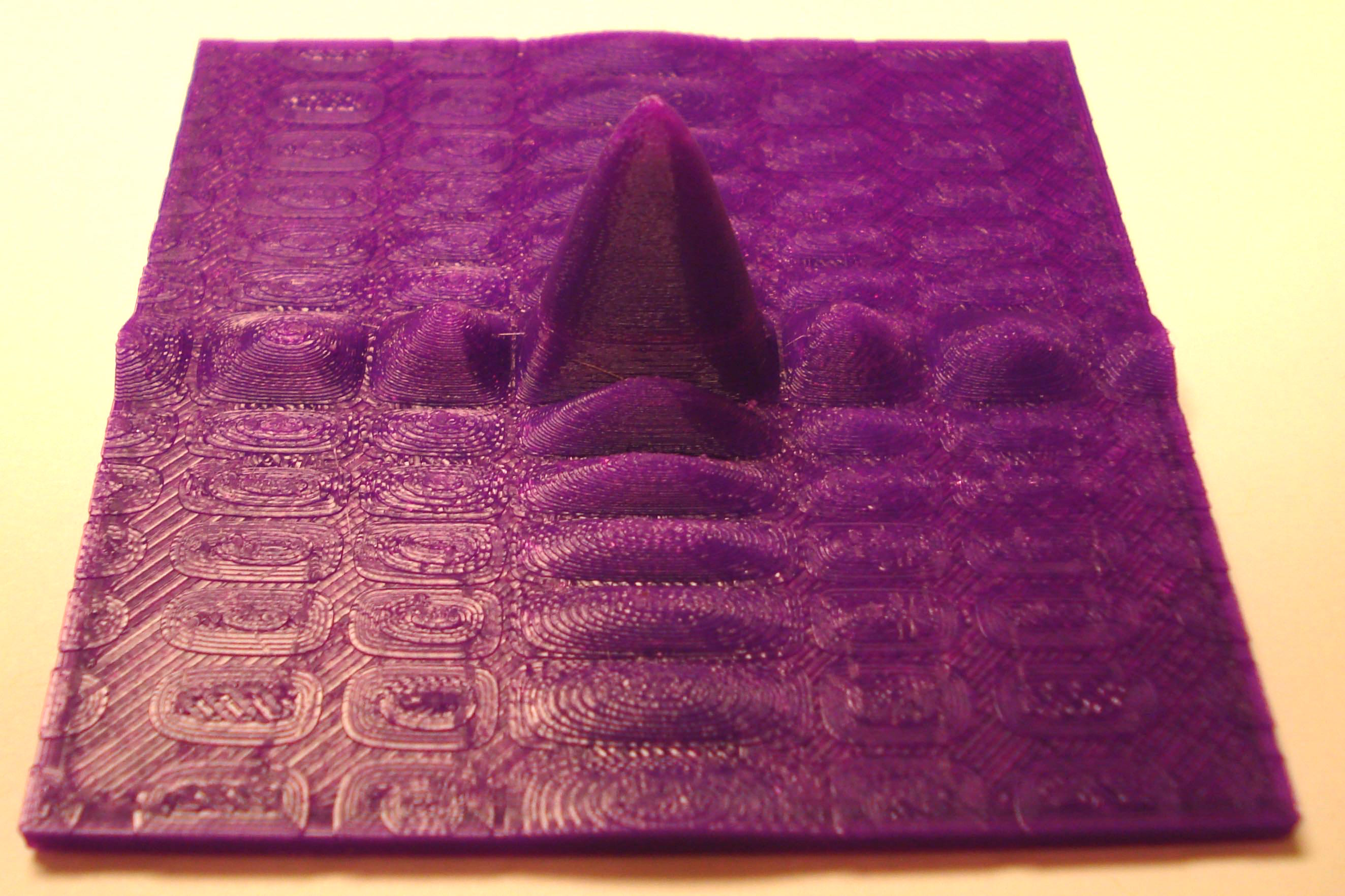
Here are two Fraunhofer diffraction intensity pattern files that have been calculated using MatLAB. The first is for diffraction from a circular aperture and printed as approximately perceived by the eye. The second file is for diffraction from a rectangular aperture and printed as approximately perceived by the eye. Since the eye has a somewhat logarithmic response to the intensity of light, these patterns are the square root of the calculated intensity, this brings out the detail and is equivalent to "overexposing" the film.
Files to download:
Circular diffraction .stl file.
This model may be printed at any size.Rectangular diffraction .stl file.
This model may be printed at any size.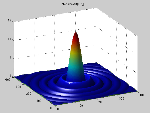 bessel3d.m MatLAB code
to plot diffraction from a circular aperture.
bessel3d.m MatLAB code
to plot diffraction from a circular aperture.This MatLAB code uses the stlwrite and surf2solid functions by Sven Holcombe. Instructions for exporting stl files from MatLAB.
-
 Circular aperture .3dremel.zip (zipped Dremel Idea Builder file) scaled to 8 cm by 8 cm
 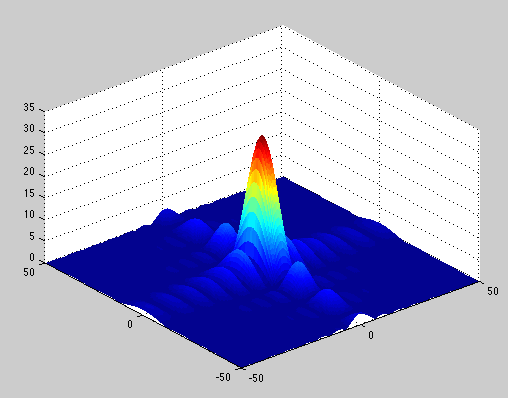 rectaperture.m MatLAB code to plot diffraction from a rectangular aperture.
This MatLAB code uses the stlwrite and surf2solid functions by Sven Holcombe. Instructions for exporting stl files from MatLAB.
 Rectangular aperture .3dremel.zip (zipped Dremel Idea Builder file) scaled to 8 cm by 8 cm
Build time for these are approximately 1 hr each.
Wave Patterns for Red and Blue Light
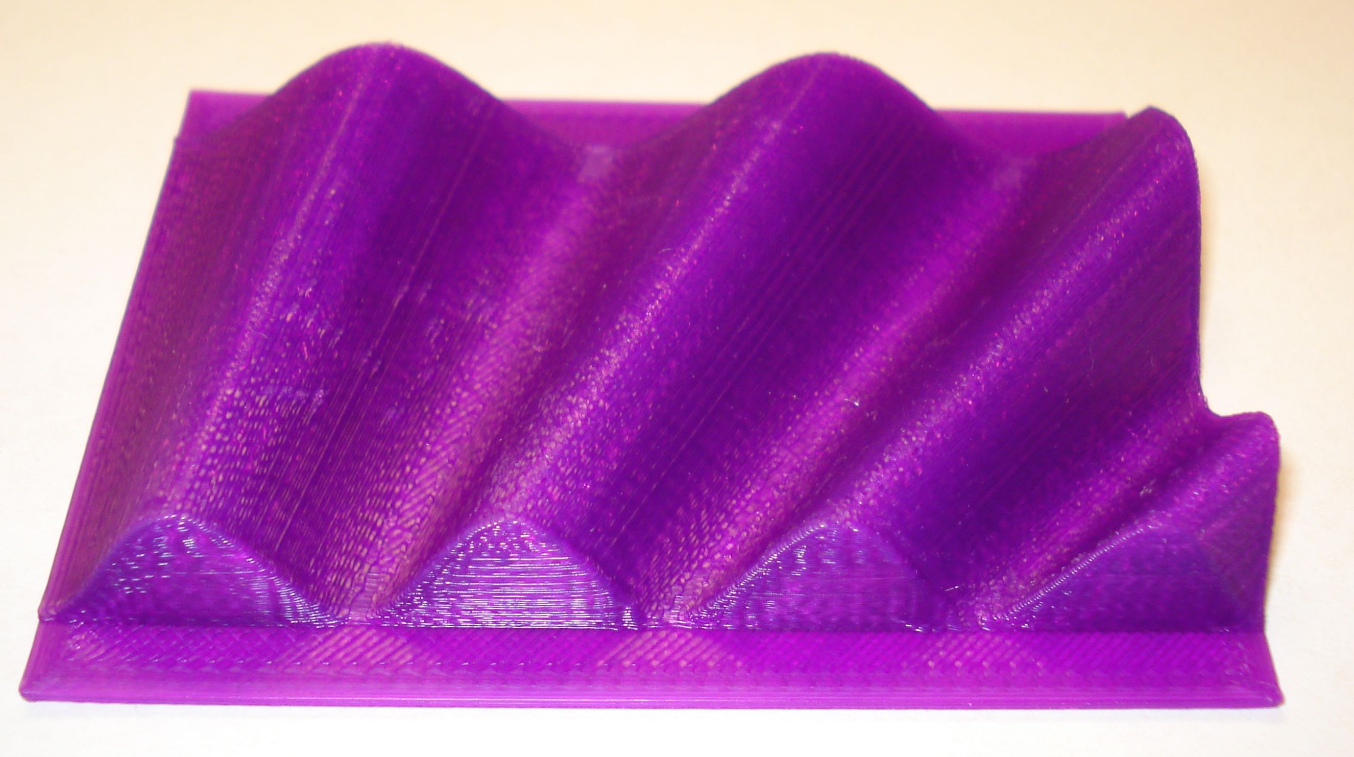
Here are two wave pattern files that have been calculated using MatLAB. The visual range of light is from 400 nm to 700 nm. The first object represents a blue light (400 nm) wave next to a red light (700 nm) wave to gain an understanding of the difference in the wavelengths. The second object represents a continuous change in the wavelengths from 400 nm to 700 nm.
Files to download:
Red-Blue waves .stl file.
This model may be printed at any size.Continuous change Red to Blue wave .stl file.
This model may be printed at any size.-
 rbwave.m MatLAB code to plot the two waves side by side.
This MatLAB code uses the stlwrite and surf2solid functions by Sven Holcombe. Instructions for exporting stl files from MatLAB.
-
 Red-Blue waves .3dremel.zip (zipped Dremel Idea Builder file) scaled to 8 cm by 8 cm
 -
 rbwave.m MatLAB code to plot a continuous change in the wavelength from 400 to 700 nm.
This MatLAB code uses the stlwrite and surf2solid functions by Sven Holcombe. Instructions for exporting stl files from MatLAB.
-
 Continuous change Red to Blue wave .3dremel.zip (zipped Dremel Idea Builder file) scaled to 8 cm by 8 cm
Build time for these are approximately 1 hr each.
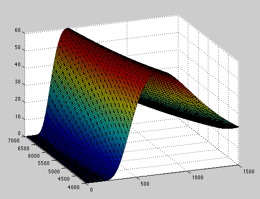
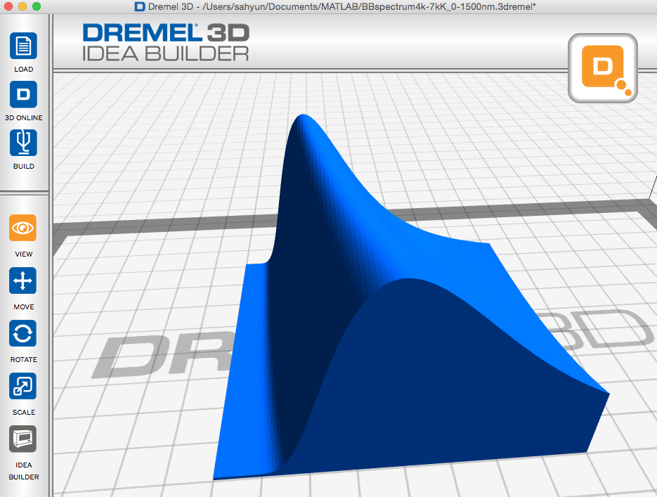
Plank Blackbody Spectra
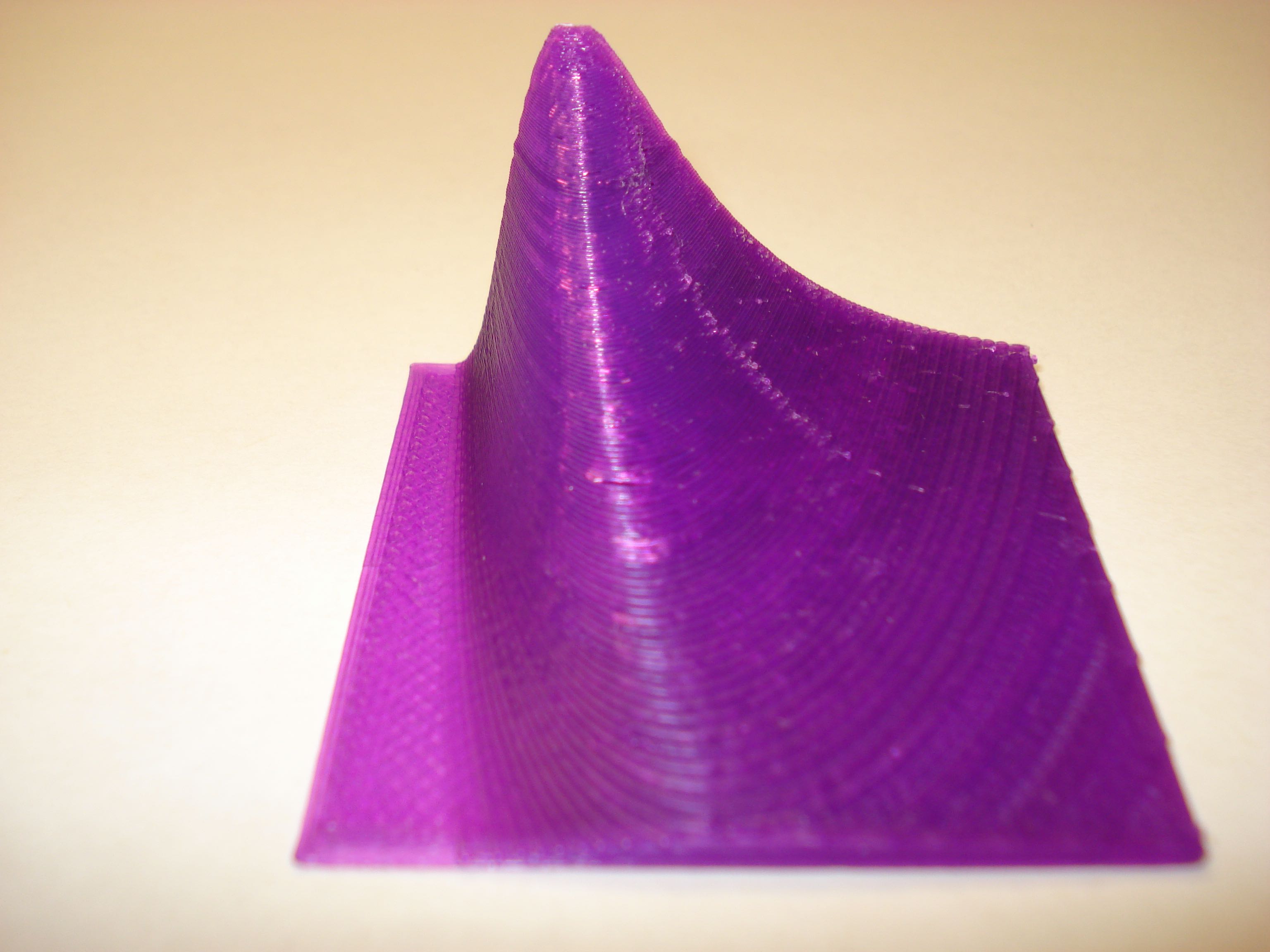
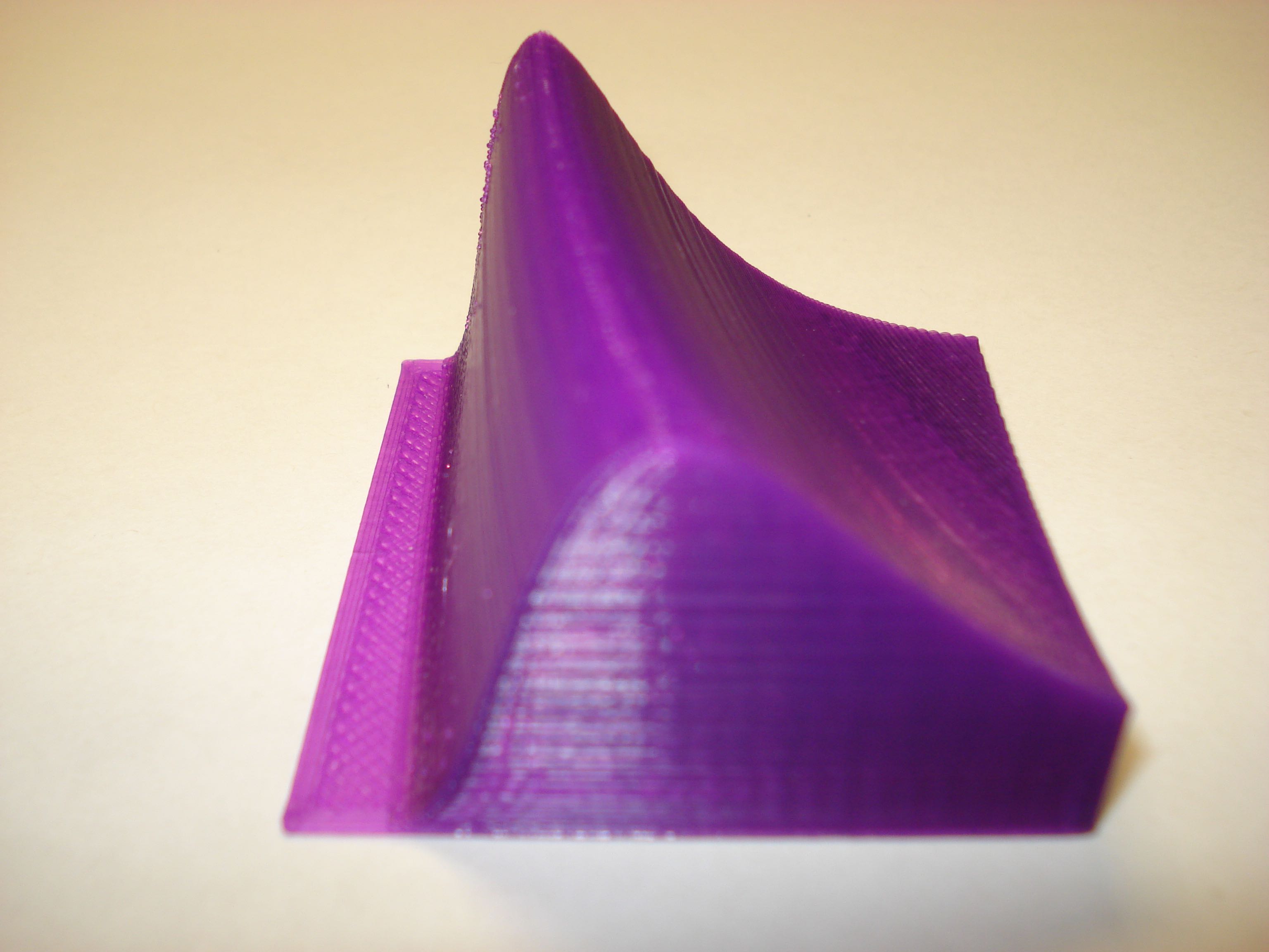
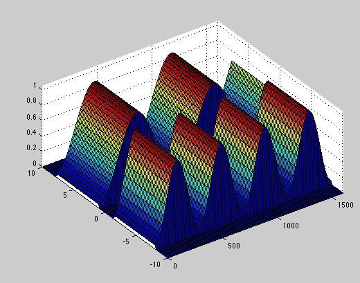
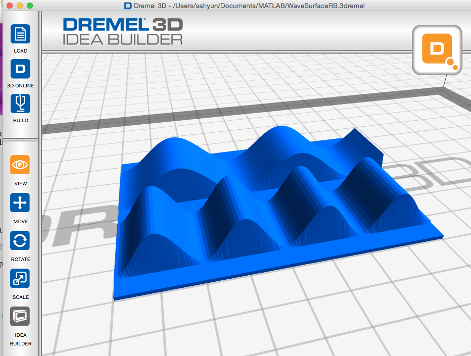
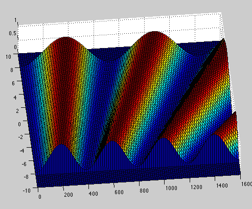
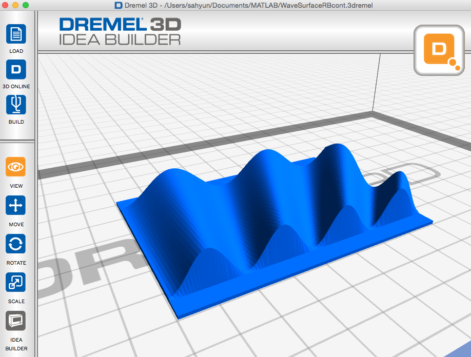
Here are Plank Blackbody Radiation spectra over a range of temperatures that have been calculated using MatLAB. The displayed prints are for wavelengths from 0 to 1500 nm and for temperatures from 4000 K to 7000 K. The first object shows the relative intensity changes between the spectra; the second print represents equal (scaled) maximum intensity curves so curve shape and peak intensity wavelength can be more easily compared.
Files to download:
Plank Blackbody spectra .stl file.
This model may be printed at any size.Plank Blackbody spectra .stl file.
This model may be printed at any size.-
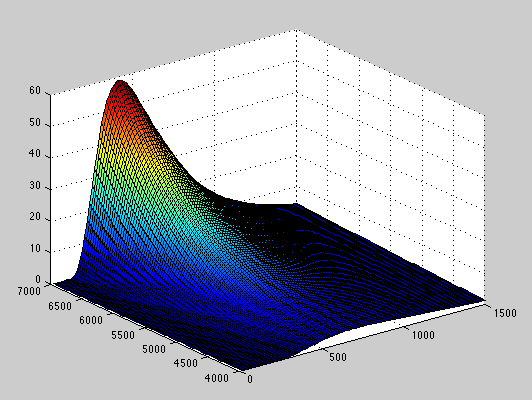 plankBB3d.m MatLAB code to plot the Plank Blackbody spectra over a range of wavelengths and temperatures.
This MatLAB code uses the stlwrite and surf2solid functions by Sven Holcombe. Instructions for exporting stl files from MatLAB.
-
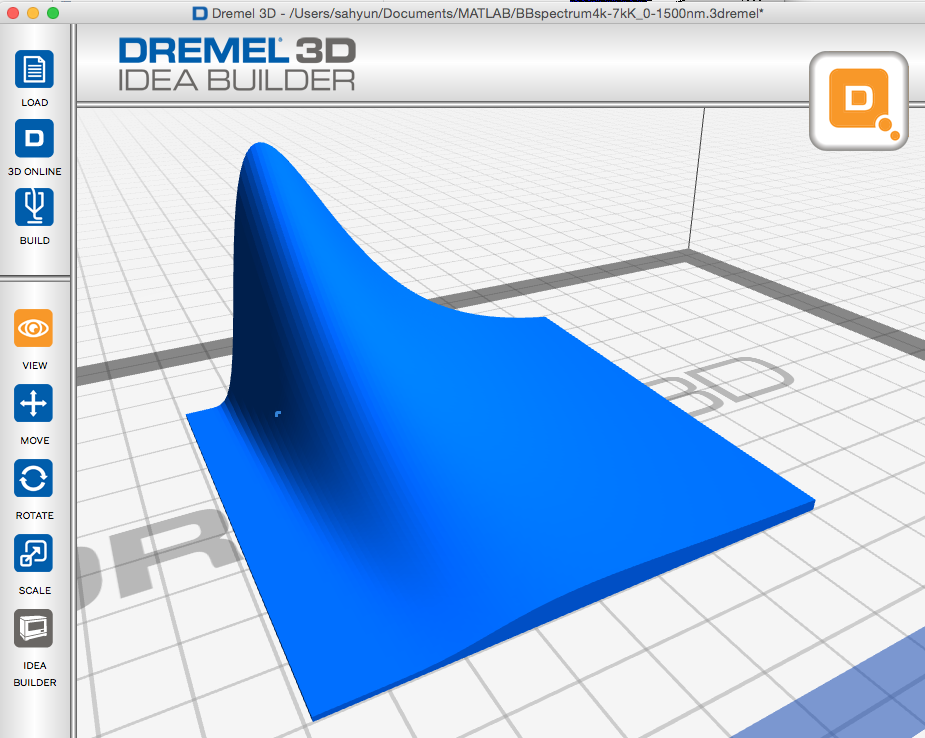 Plank Blackbody spectra .3dremel.zip (zipped Dremel Idea Builder file) scaled to 5 cm by 5 cm.
 -
 plankBB3dnorm.m MatLAB code to plot a scaled set of the Plank Blackbody spectra over a range of wavelengths and temperatures so that each curve has the same peak intensity.
This MatLAB code uses the stlwrite and surf2solid functions by Sven Holcombe. Instructions for exporting stl files from MatLAB.
-
 Plank Blackbody spectra .3dremel.zip (zipped Dremel Idea Builder file) scaled to 5 cm by 5 cm.
Build time for these are approximately 45 min. each.
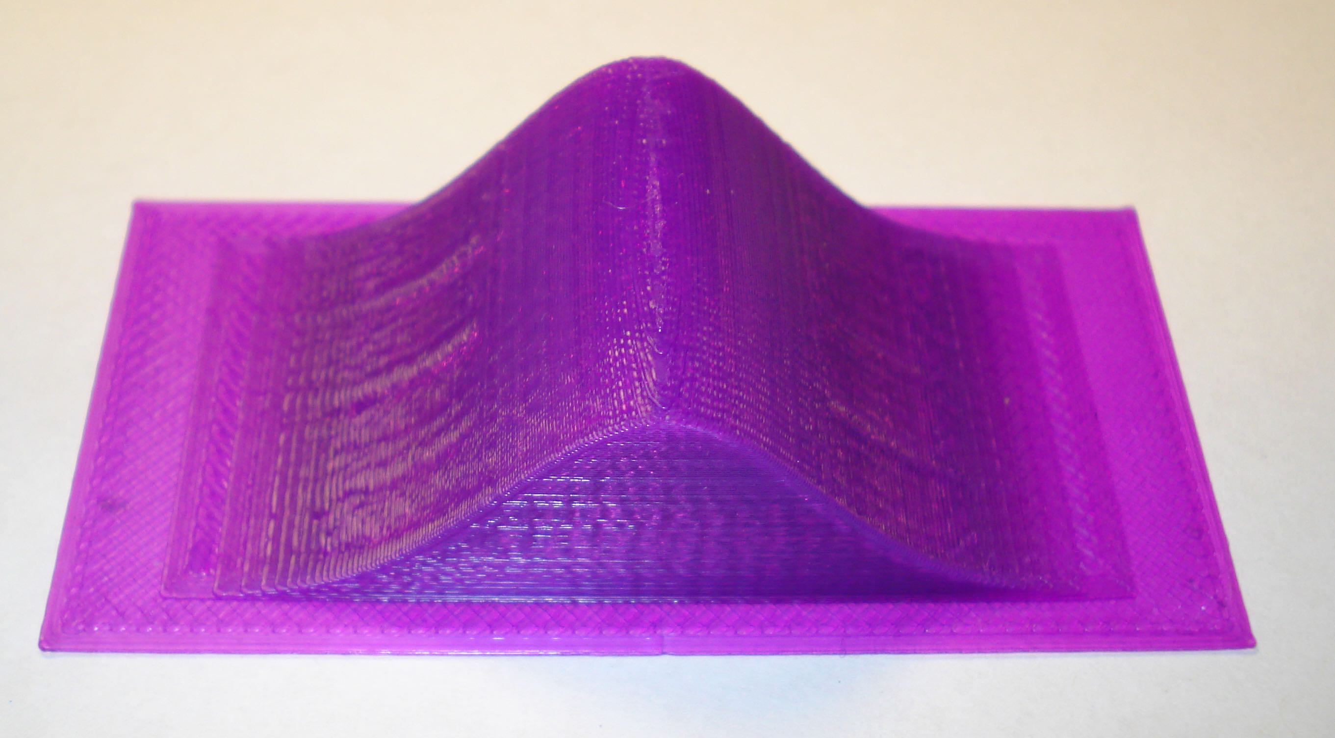
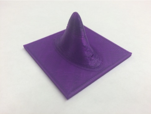
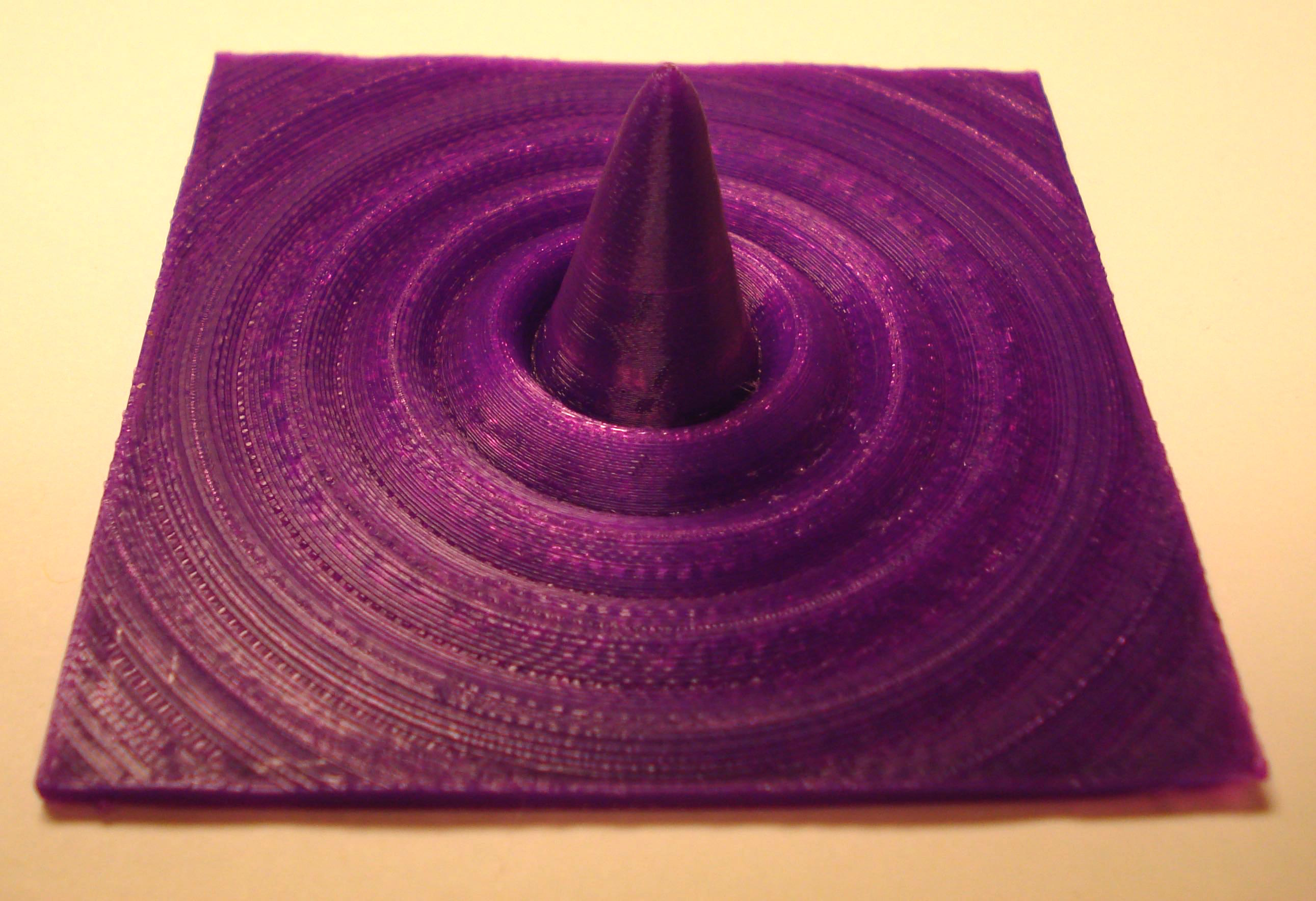
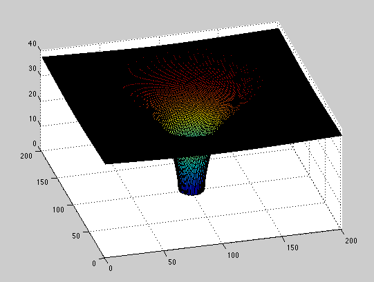
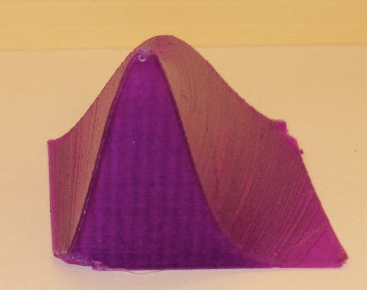
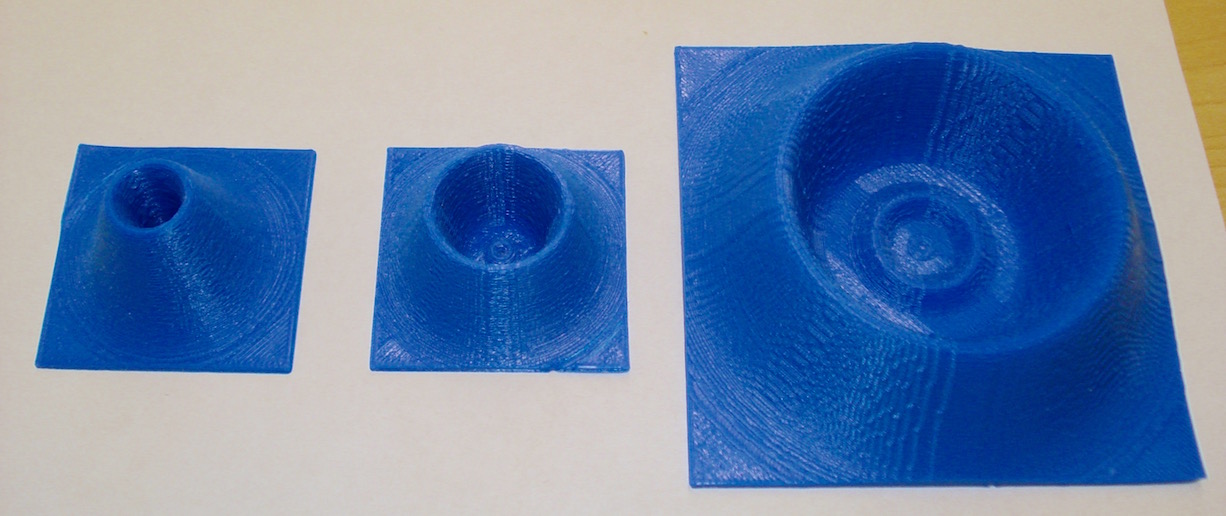
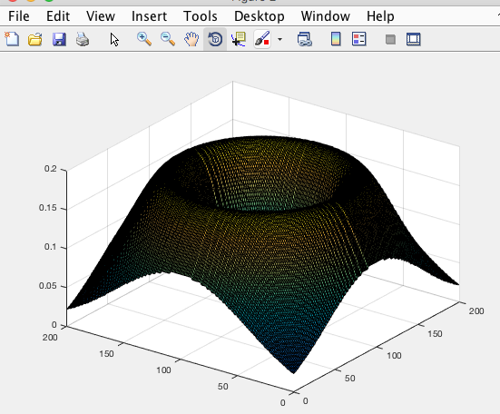
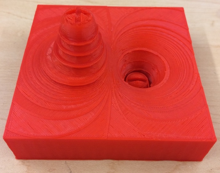
Gravitational Potential Well
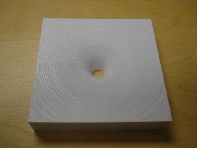
Here is a Gravitational Potential well that would be produced by mass and calculated using MatLAB. The surface represents how space is deformed by a massive object. If the object were a point mass, the result will be a Black Hole. This surface shows the Black Hole's event horizon as a circle in the bottom of the model. If this model is printed at a size of 20 cm the central hole will have a 2 cm diameter which is the size of the event horizon if the Earth were compressed to a point mass. However, for a more reasonable print time, I recommend a size of 10 cm (the central hole will have a 1 cm diameter, representing a Black hole produced by half the Earth's mass.)
Files to download:
Gravitational Potential well .stl file.
This model may be printed at any size. 10 cm recommended.-
 gravity.m MatLAB code to plot the gravitational potential well.
This MatLAB code uses the stlwrite and surf2solid functions by Sven Holcombe. Instructions for exporting stl files from MatLAB.
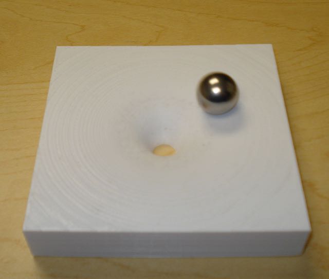
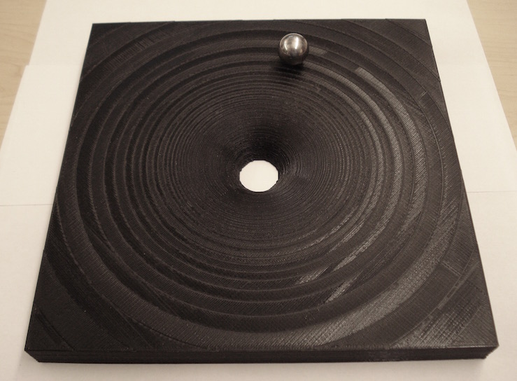
Build time at 10x10x2 cm with 0.2 mm layers and 20% (white, left) fill is approximately 5 hrs. A 20x20x2 cm print (black, right) takes approximately 20 hours but produces a model that is much easer to demonstrate an orbiting ball on.
When printed, a steel ball can be made to orbit the central hole. The larger the print size, the more easily it is to get the ball to orbit.
Bravais Cubic Lattices
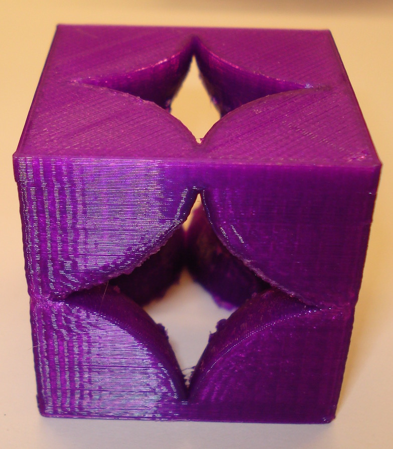
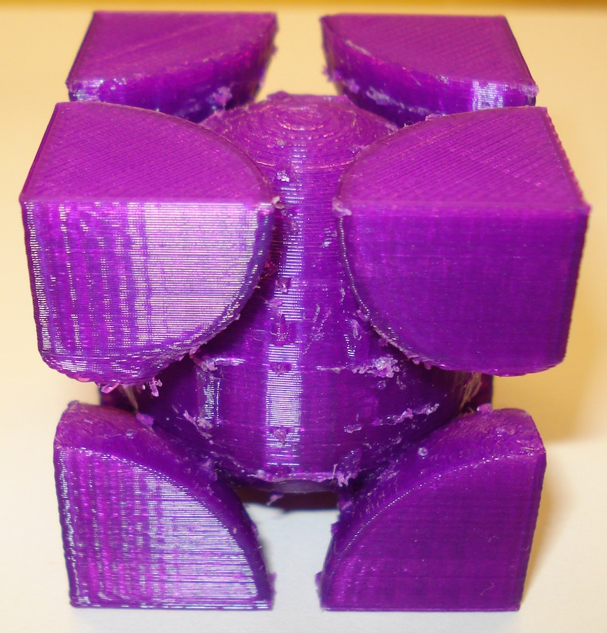
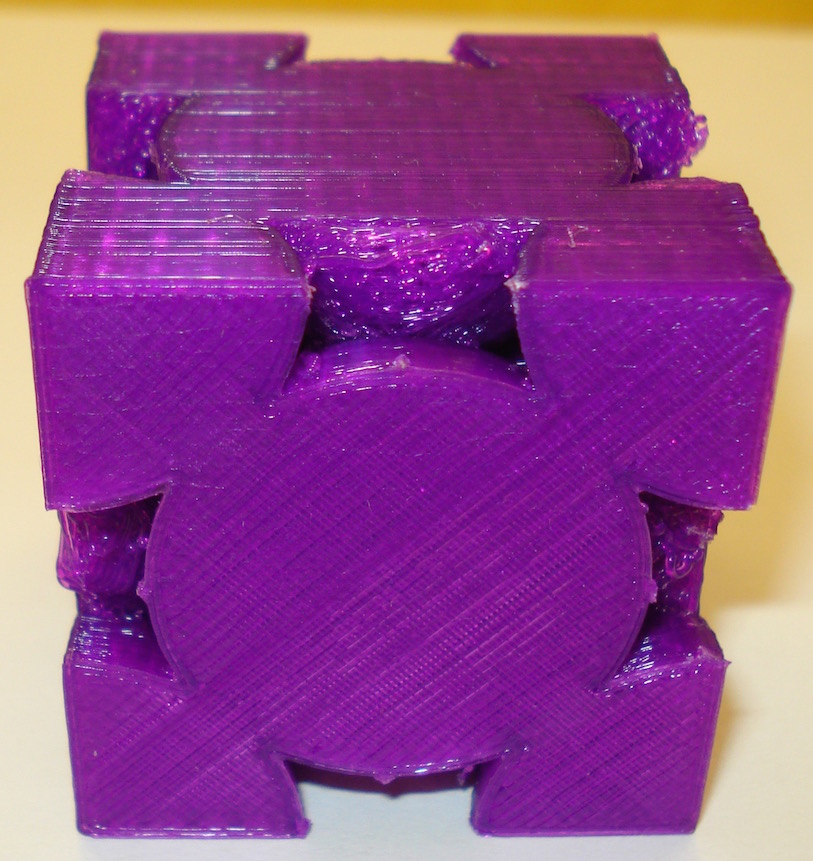
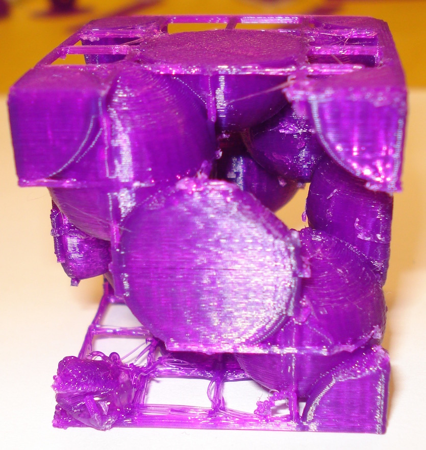
Here are four Bravais Cubic Lattice unit cells: simple cubic, body centered cubic, face centered cubic, and a diamond lattice. The simple cubic unit cell contains eight one-eighth atoms arranged each at a corner so each unit cell contains "one" atom. The Body Centered Cubic unit cell has the eight corners and a complete atom in the center so it consists of two atoms. The face centered unit cell has the eight corners and six half-atoms, one on each of the cube's sides for a total of four atoms. The diamond lattice has the eight corners, six half atoms and four internal atoms for a total of eight atoms. These models were produced using OpenSCAD. There are two versions of these cells, a "supports" version, that has a printing support structure of horizontal and vertical bars to aid in printing (and in the case of the diamond lattice, the supports are needed to connect four free corner (eighth) atoms to the model). Most of these supports can be removed after printing. A non-suport version is also available if your printer is able to provide some sort of adequate support structure.
Files to download:
Bravais cubic unit cells with supports .stl.zip file.
This is a .zip archive containing a Simple Cubic, Body Centered Cubic, Face Centered Cubic, and Diamond Bravais lattice unit cell models with support structure to aid in printing. They may be printed at any size. 4 cm recommended.Bravais cubic unit cells .stl.zip file.
This is a .zip archive containing a Simple Cubic, Body Centered Cubic, Face Centered Cubic, and Diamond Bravais lattice unit cell models. Some sort of support structure will need to be added for successful printing (especially with the Diamond lattice!) They may be printed at any size. 4 cm recommended.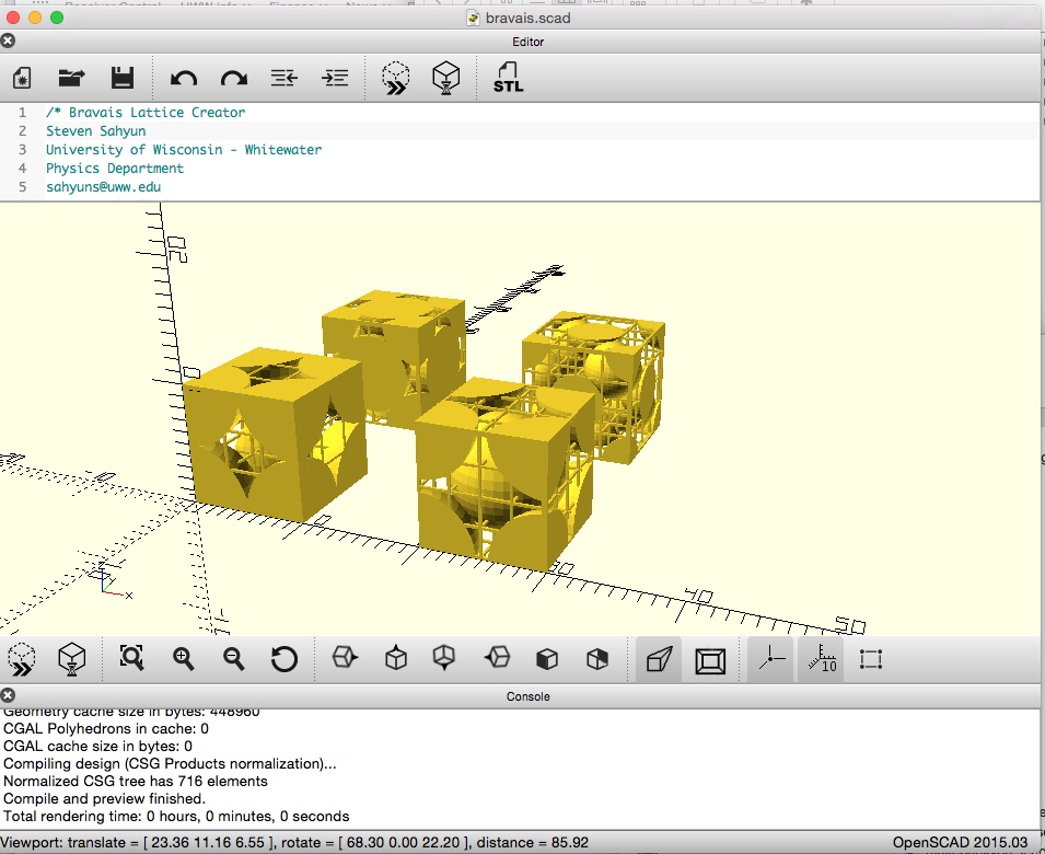 Bravais cubic unit cells OpenSCAD code. This is the OpenSCAD file used to generate these unit cells. You can adjust the support structure and select unit cells.
Bravais Lattice Unit Cells
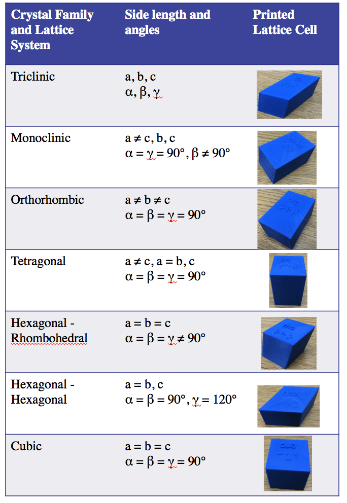
Here is a set of the seven Bavais Lattice geometric figures cells. The unit cells are: Triclinic, Monoclinic, Orthorhombic, Tetragonal, Hexangonal, Rhombohedral, and Cubic. These are solid unit cell representations of the crystal unit cells. Each cell has text and braille labeling.
Files to download:
Bravais set .stl.zip file.
This is a .zip archive containing the set of the seven Bravais unit cells: Triclinic, Monoclinic, Orthorhombic, Tetragonal, Hexangonal, Rhombohedral, and Cubic.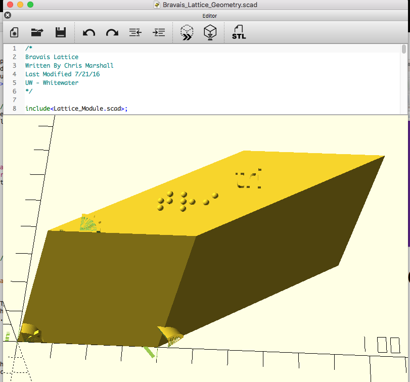 Bravais unit cells OpenSCAD code .zip There are two files in this .zip archive: Bravais_Lattics_Geometry.scad and Lattice_Module.scad that are used to generate these unit cells. Created by Christopher Marshall
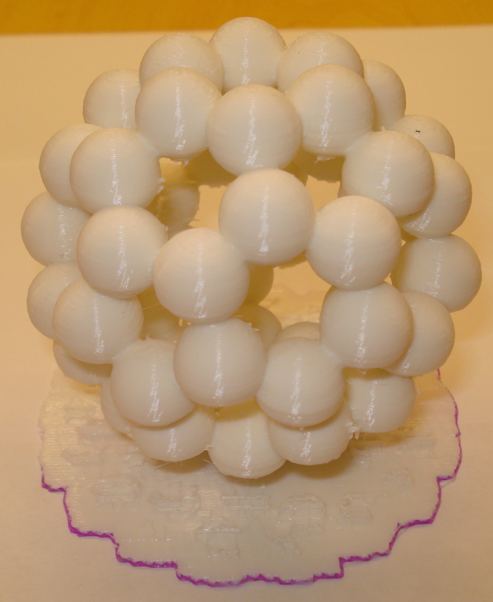
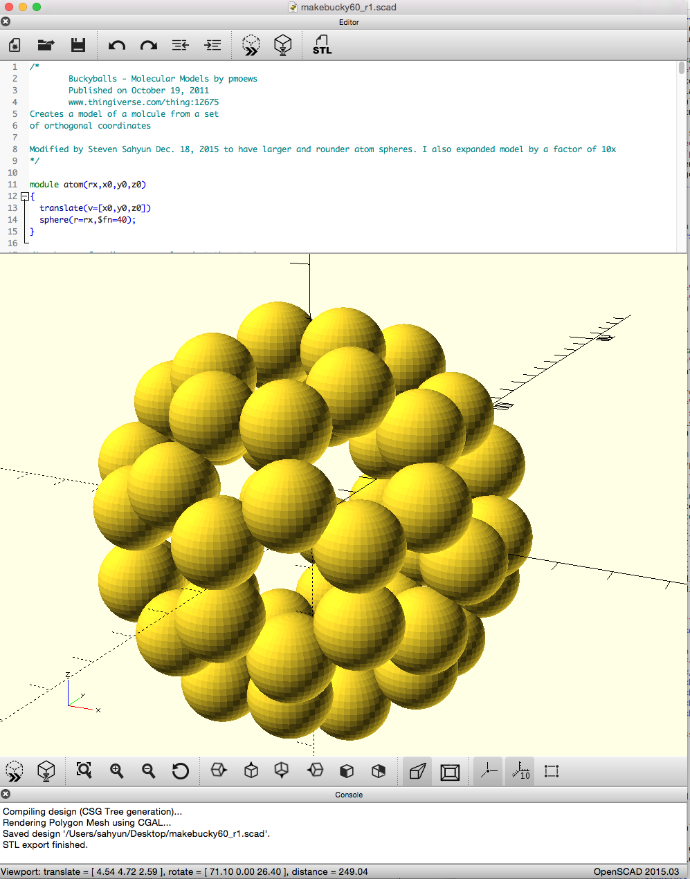
Carbon-60 Molecule (Buckyball)
Files to download:
Carbon-60 molecule .stl file.
This model may be printed at any size. 10 cm recommended.-
 Bucky60.stl OpenSCAD code to plot the Carbon-60 Buckyball model.
This is a modification of pmoews' Carbon 60 molecule found on Thingiverse.
Buckyballs - Molecular Models by pmoews
Published on October 19, 2011
www.thingiverse.com/thing:12675
Creative Commons - Attribution
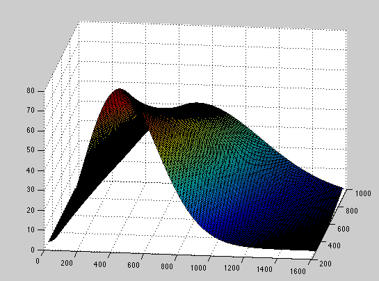
Thermal Distribution of Molecular Speeds
This is the Maxwell distribution of the speed of molecules in an ideal gas for a range of temperatures. The equation is The plotted speed (x-axis) varies from 0 to 1600 m/s while the temperature (y-axis) ranges from 300 to 900 Kelvin. Plot produced by Dan Marzahl and Steven Sahyun.
Files to download:
Gas Speed Distribution .stl file.
This model may be printed at any size. 5 cm recommended.-
 gas_speed_distribution.m MatLAB code to plot the Maxwell speed distribution.
This MatLAB code uses the stlwrite and surf2solid functions by Sven Holcombe. Instructions for exporting stl files from MatLAB.
Equal Torque Lever
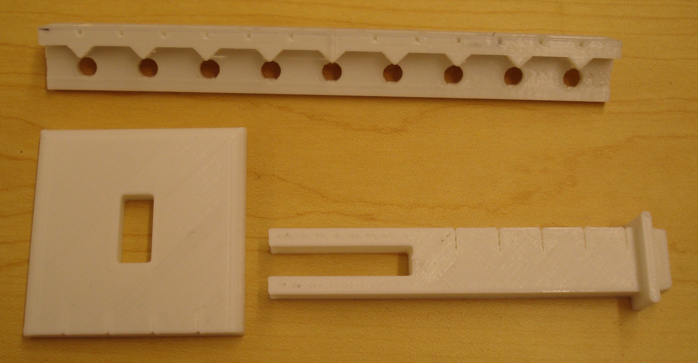
This is a balancing lever system for learning about torques (τ = r ⨯ F = rFsinθ) in equilibrium.. This object consists of a base plate, a support beam and a lever beam. Features include tactile marks in the center of the lever to easily find the middle and 9 fulcrums and 9 hanging holes to provide a range of options for investigating torques. There are bins on the top of the lever to allow for fine balancing adjustments if needed. There are centimeter markings on all objects so printing scale can be coordinated. Lever designed by Chris Marshall and Steven Sahyun.
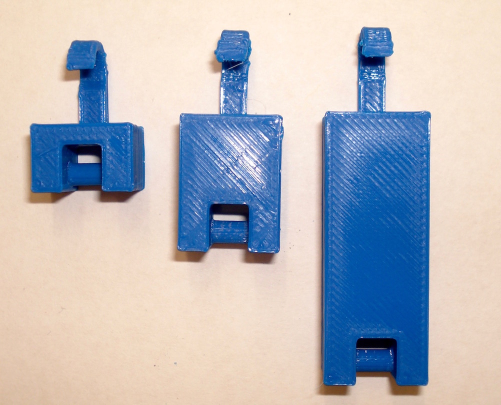
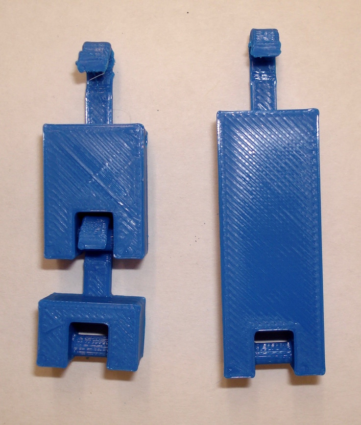
Also available is a mass set with 1, 2, and 4 mass unit blocks that hang from the holes on the lever. The masses can be connected to provide more arrangements.
Files to download:
Lever .stl file.
This model should scale correctly in your 3D program.Hanging mass set .stl file.
This model should scale correctly in your 3D program.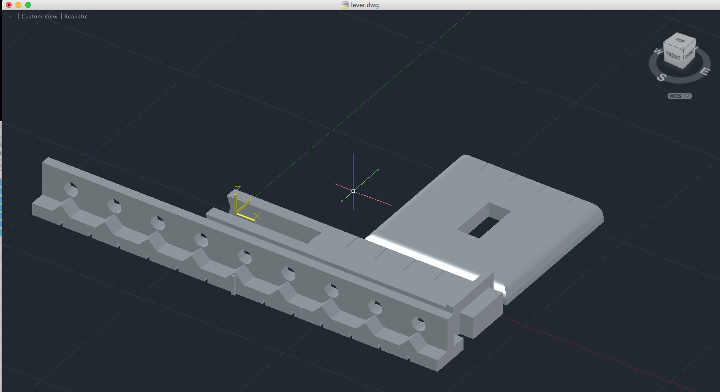 Lever .dwg.zip (zipped AutoCAD file.)
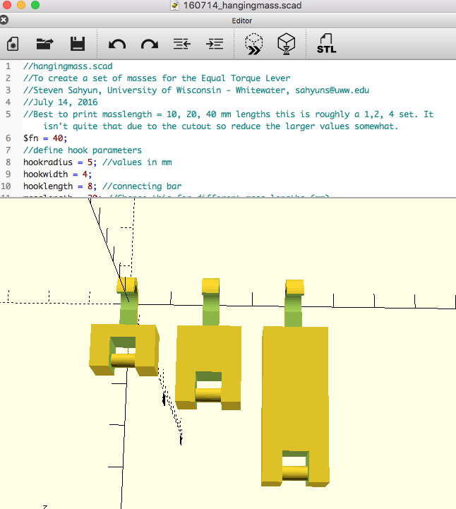 Hanging Mass Set .scad.zip (zipped OpenSCAD file.)
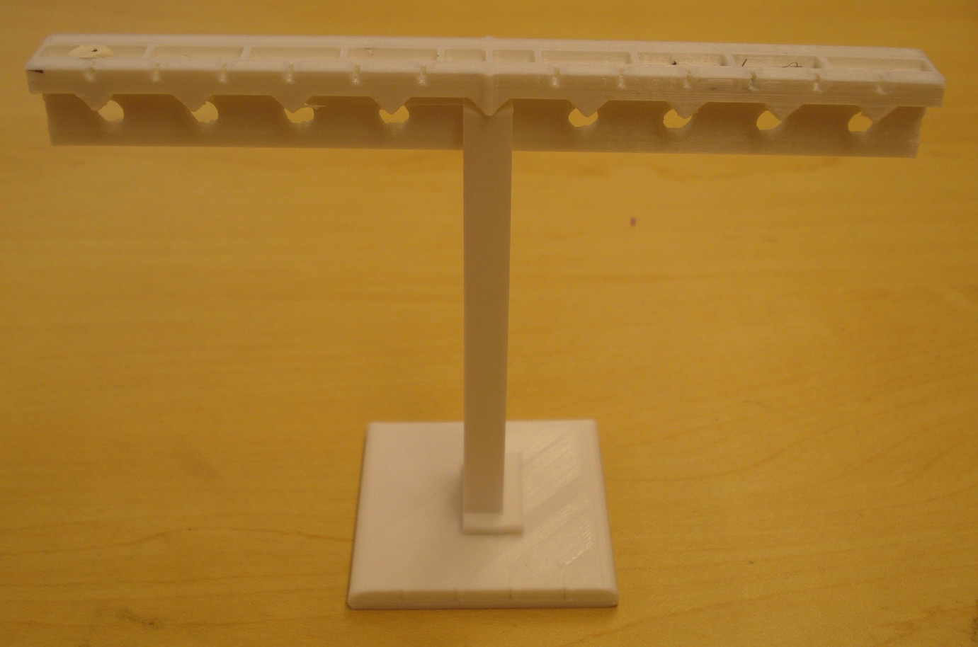
Here the lever is shown with the 2 and 4 mass units.
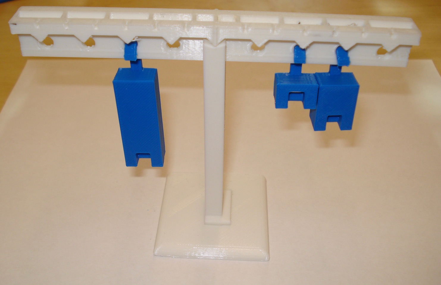
Here the lever is shown with the 1, 2 and 4 mass units. On the left the 4 unit mass is 2 distance units so 2x4 = 8. On the right, the 1 unit mass is 2 distance units and the two unit mass is three distance units so 1x2+2x3 = 8 and the torques balance.
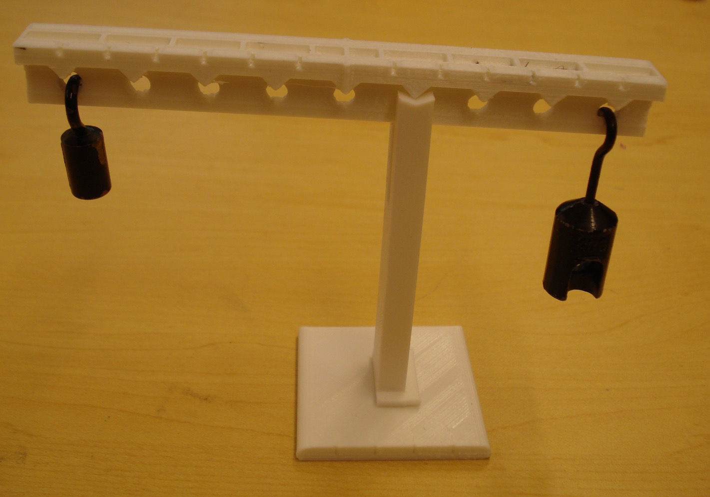
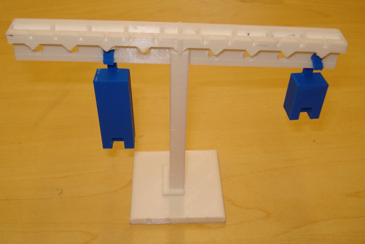
Here the lever is shown with a 10 g mass on one end (Ll = 5 units) and a 20 g mass on the other end (Lr = 3 units) which are approximately equal (50 g units ≅ 60 g units). Note: the finite mass of the lever accounts for the missing 10 g units.
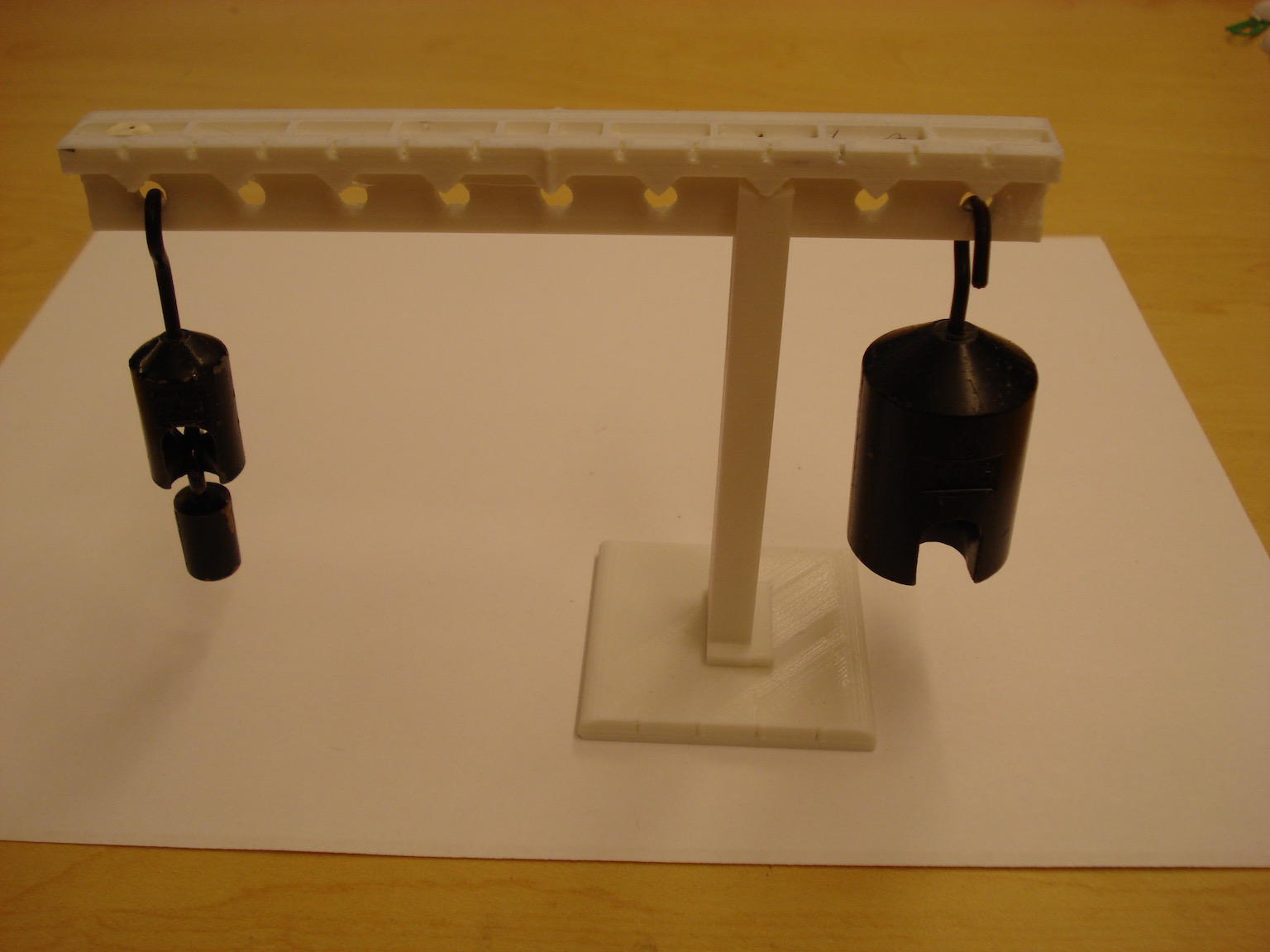
Here the lever is shown with 30 g of mass on one end (Ll = 6 units) and a 100 g mass on the other end (Lr = 2 units) which are approximately equal (180 g units ≅ 200 g units). Note: the finite mass of the lever accounts for the missing 20 g units.
Back to top of page.Protractor
(Updated August 8, 2017)
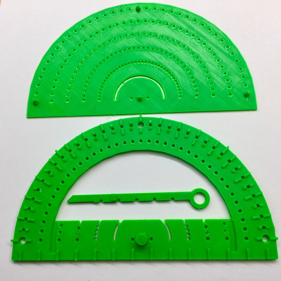
This protractor allows students and their teachers to create tactile angles using a standard braille stylus or pen in order to make marks on paper. Our design comes with a base plate similar to that of a braille slate, with pegs that stick through a piece of paper to lock the protractor in place. The protractor can then be used to draw angles. The protracor has markings every 5 degrees and a pointer to guide the drawing and measurement of angles. There are larger marks every 10 degrees with additional indicators at 0, 45, 90, 135, and 180 degrees. There are marking holes, guide marks in the angle pointer, and the base plate has divots to help with markng angles. This protractor also includes a centimeter ruler along the base. Protractor designed by Steven Sahyun.
This model has been uploaded to YouMagine as: Tactile Protractor
Files to download:
Protractor with pointer and base plate .stl file.
This model should scale correctly in your 3D program.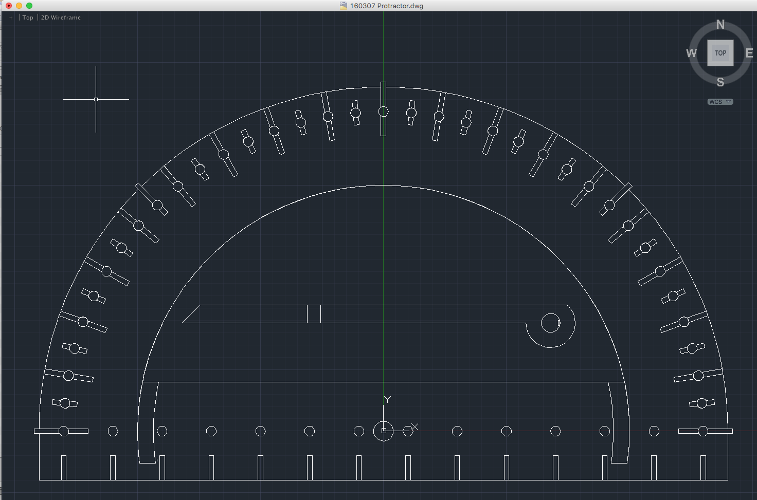 Protractor .dwg.zip (zipped AutoCAD file.)
How to use this protractor.
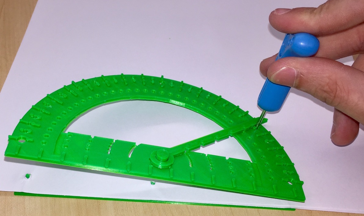
To use this protractor, start by placing the bottom on the underside of a piece of paper. The pegs on the base plate will stick up through the paper, and the top can then be fitted over those pegs. Now, simply snap the pointer into place, and away you go! The pointer has marks in it that allow the user to measure angles with more precision, and holes in the protractor allow the drawing of lines and arcs.
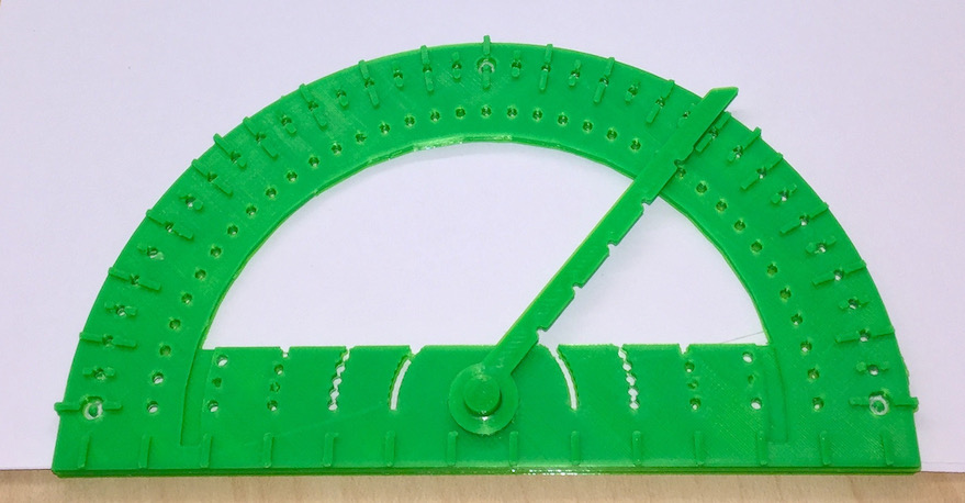
Next, set the pointer to the desired angle. The pointer fits between the 5 and 10 degree markings to act as a useful guide. The 5 degree markings are inset so you can easily feel between adjacent angle markings such as 15 and 20 degrees. The holes for the stylus are in the center of the marks. Note that the 0, 45, 90, 135, and 180 degree marks are extended so they can be easily located. Mark the angle on the inside area of the protractor (there are five additional locations along the pointer) and on the outer edge where the pointer is near the angle marks.
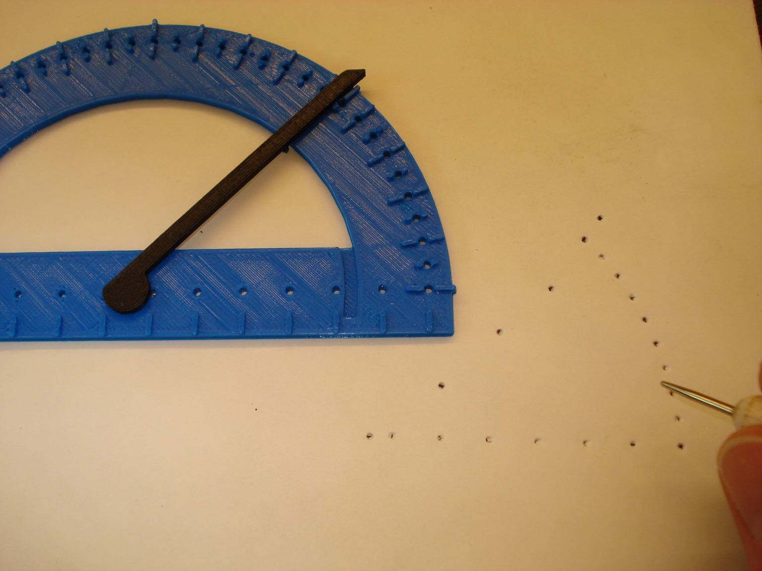
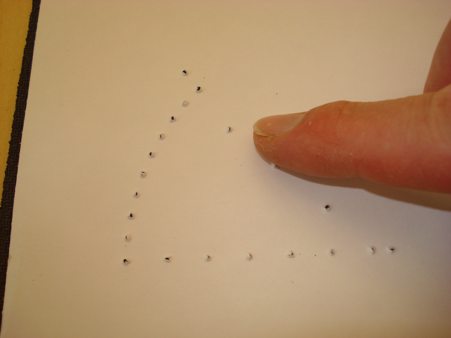
The angle has now been marked and when the protractor is removed, the paper retains the indented markings. Turn the paper over and the tactile angle is easily felt.
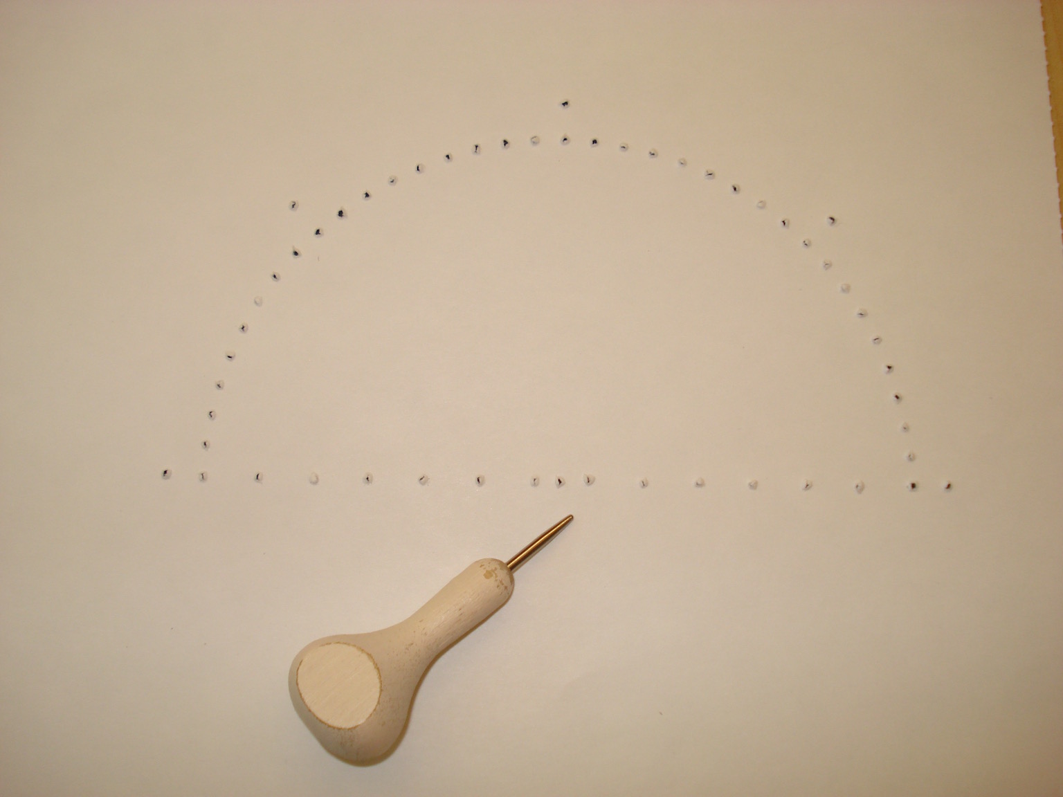
A tactile 180 degree semi-circle with marks every 5 degrees and additional marks at 0, 45, 90, 135, and 180 degrees is easily constructed with this protractor. The base is marked with rulings spaced 1 cm apart with an extra mark at the circle's center.
Back to top of page.Hydrogen Electron Radial Probability (S, P, D, F)
1S, 2S and 3S Radial Probability:
2P, 3P Radial Probability:
3D Radial Probability
These objects are Hydrogen Radial Probability through the xz-plane for several quantum values. Note that the region of highest probability corresponds to the classical Bohr radius. However, the radial probability values u2 are not the same as the maximum wavefunction value (Ψ).
Files to download:
zip archive of the 7 radial probability .stl files.
-
 MatLAB code used to calculate these surfaces..
This MatLAB code uses the stlwrite and surf2solid functions by Sven Holcombe. Instructions for exporting stl files from MatLAB.
The Hydrogen 2s radial probability graph as shown on the HyperPhysics site.
Image credits: R Nave, Hyperphysics. (2016) http://hyperphysics.phy-astr.gsu.edu/hbase/hydwf.html#c3
A typical image of the Hydrogen wavefunctions is shown on Wikipedia: 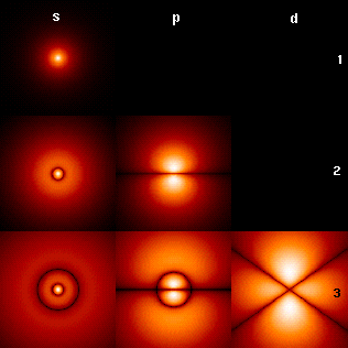
Image credits: Wikipedia, Hydrogen Atom. (2016) https://en.wikipedia.org/wiki/Hydrogen_atom
Hydrogen Electron Orbital Shells (S, P, D, F)
Here is an excellent source for the Hydrogen Isopotential Surfaces:
Do-It-Yourself: 3D Models of Hydrogenic Orbitals through 3D Printing
Kaitlyn M. Griffith, Riccardo de Cataldo, and Keir H. Fogarty
Journal of Chemical Education Article ASAP
DOI: 10.1021/acs.jchemed.6b00293
July 7, 2016
http://pubs.acs.org/doi/abs/10.1021/acs.jchemed.6b00293
The site has a link to the pdf of the paper by Griffith, deCataldo and Fogarty that has general information about printing techniques for the orbital isopotentials. The Supporting Information pdf goes into specific detail about how to create the objects, and the
ZIP archive contains a set of .stl file objects for the s, p, d, and f orbitals.
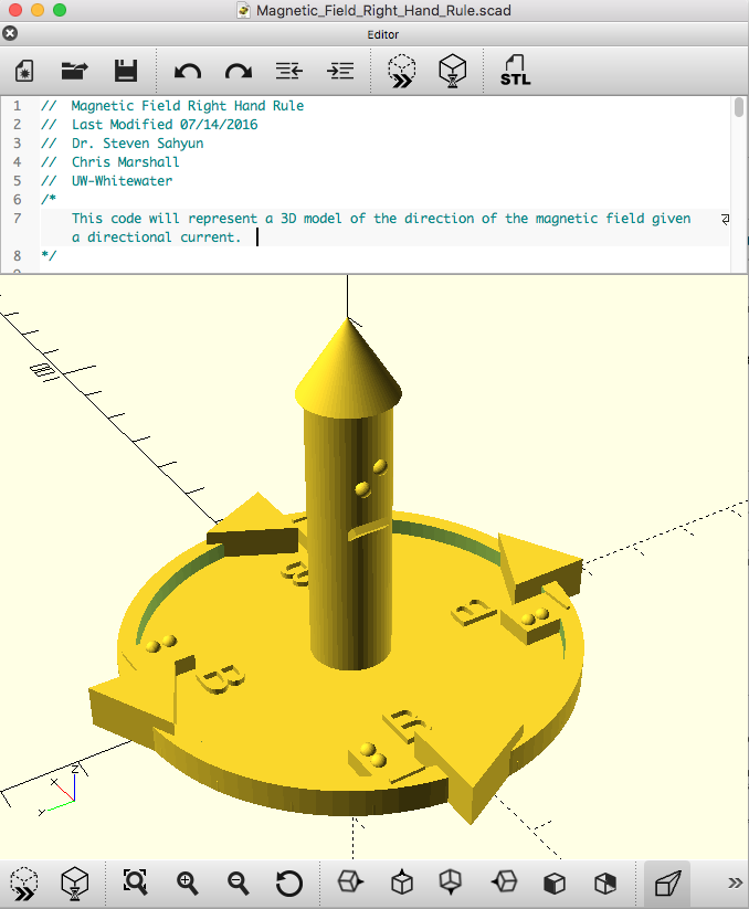
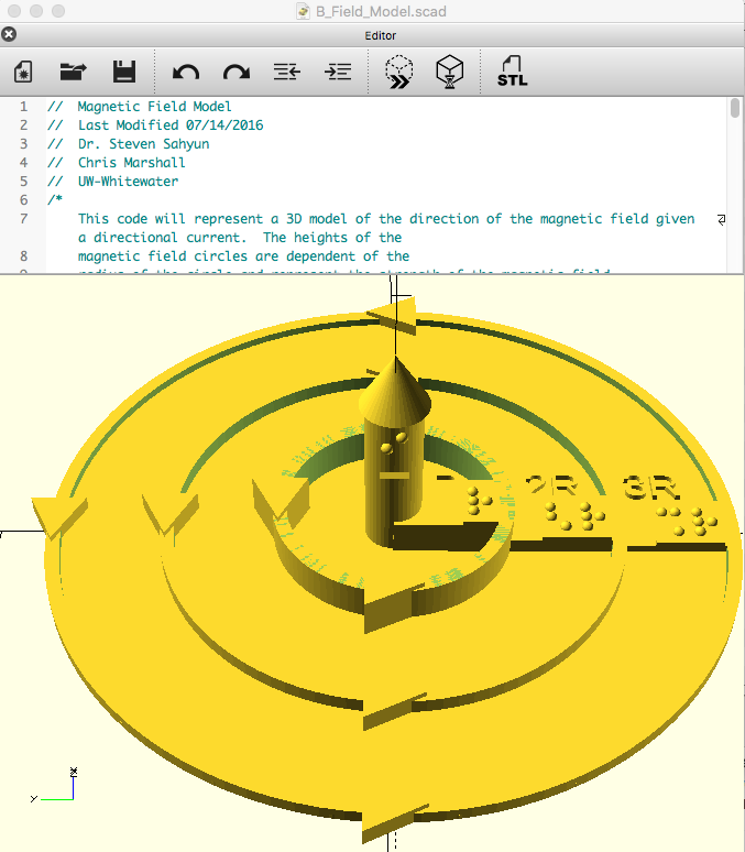
Direction of the Magnetic Field Due to a Linear Current (Right-hand rule)
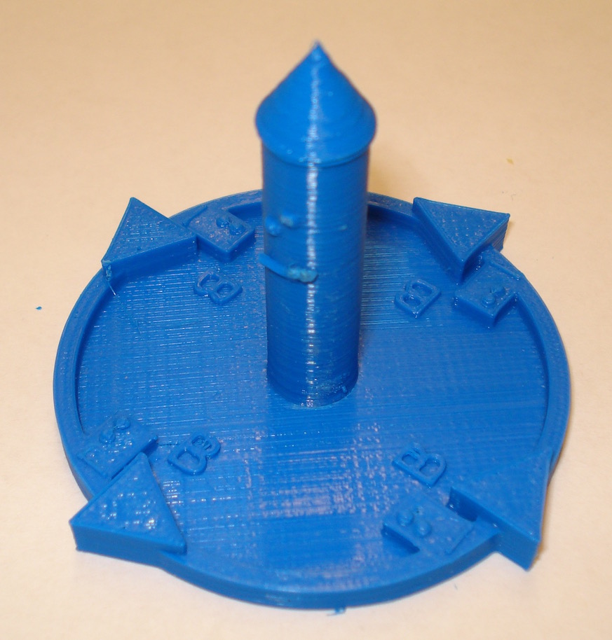
This print demonstrates the right-hand rule for the magnetic field produced from a current of strength I given by the equation B = μ0I/2πr. The current is represented by the central column with a cone to indicate the direction. The arrows indicate the direction of the magnetic field. This object has both Braille and text labels.
Files to download:
 Bfield right hand rule OpenSCAD code .scad.zip
Magnitude of the Magnetic Field Due to a Linear Current
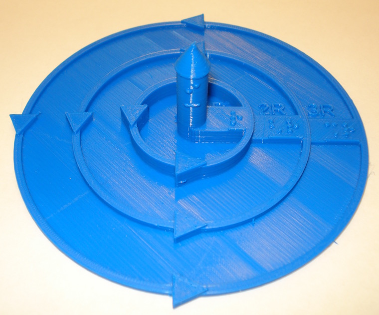
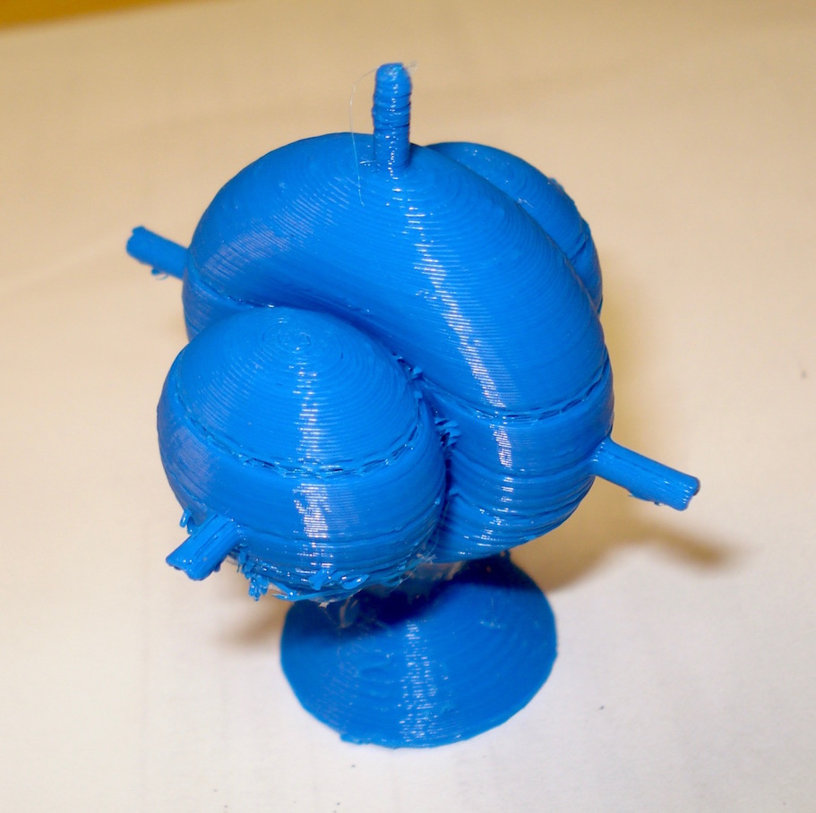
This print demonstrates how the magnitude of the magnetic field produced from a current changes with distance from I given by the equation B = μ0I/2πr. The current is represented by the central column with a cone to indicate the direction. The arrows indicate the direction of the magnetic field. The magnitude of the magnetic field at distances r, 2r and 3r are indicated by the height of the rings (1, 1/2, 1/3). This object has both GS Braille and text labels.
Files to download:
 B field magnitude OpenSCAD code .scad.zip
XYZ and IJK Coordinate Axes
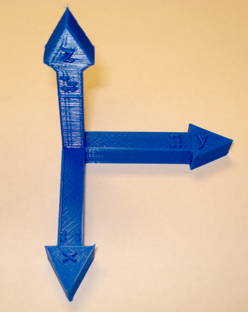
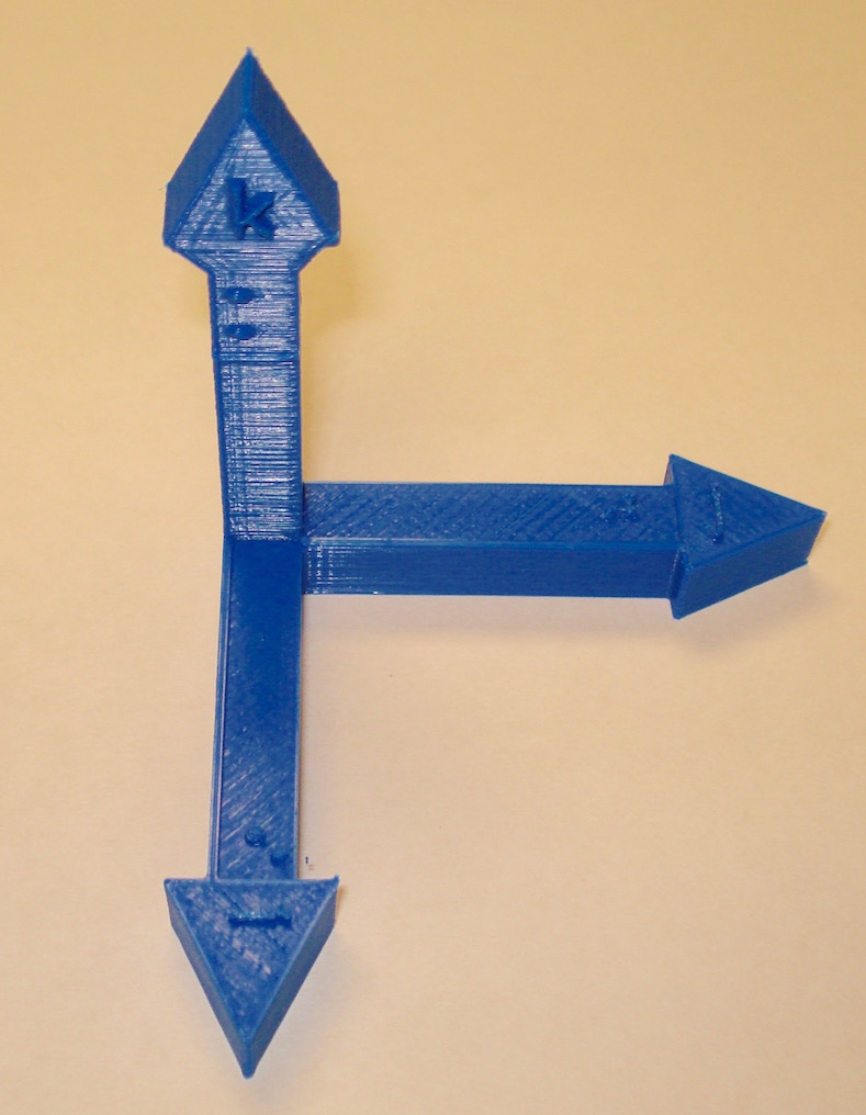
These are right-hand X-Y-Z and I-J-K coordinate axes. These objects have both Braille and text labels.
These models have been uploaded to YouMagine as: XYZ coordinate axes and IJK coordinate axes
Files to download:
XYZ coordinate .stl file.
IJK coordinate .stl file.
-
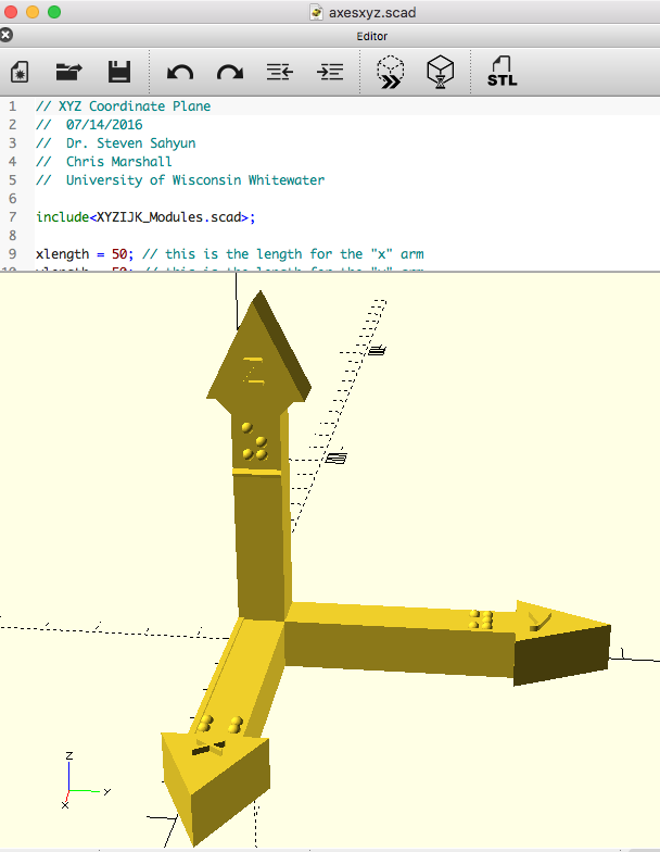
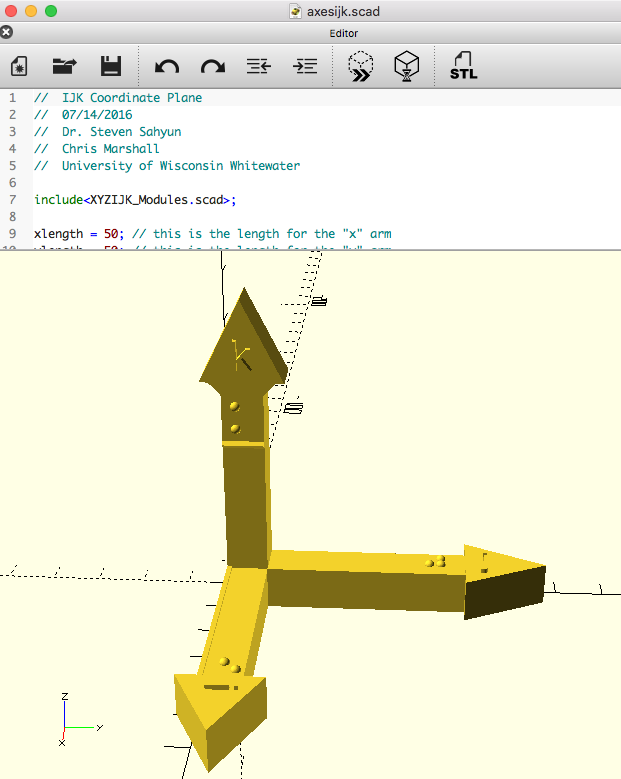 XYZ and IJK axes OpenSCAD code .scad.zip The OpenSCAD XYZ and IJK Coordinate models use modules from the XYZIJK_Modules.scad file included in the .zip archive to run. Keep both files in the same directory when using these in OpenSCAD.
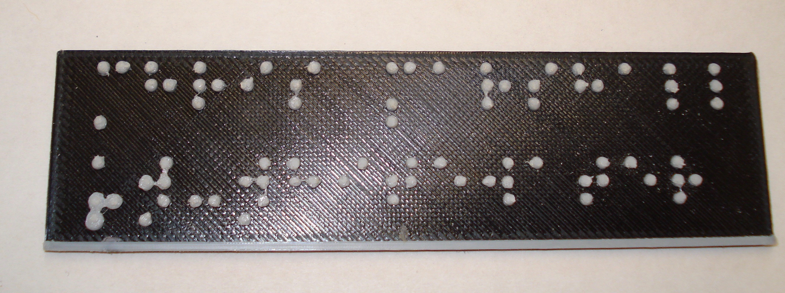
Braille Labels
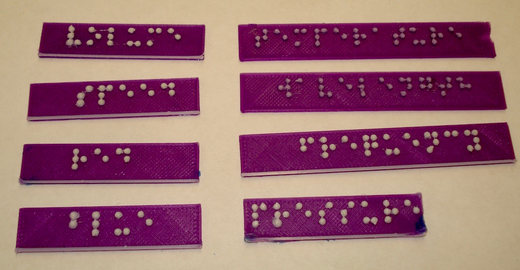
These labels were created with the Braille label maker OpenSCAD script. It may be useful to have labels for some of the objects on this site. Objects and appropriately placed labels may be glued (a hot-glue gun is particularly useful) to a base board after printing. Each label has a raised edge below the text for text orientation. The labels pictured above were printed with two high contrast colors filaments so that the braille text can more easily be seen. To do this, we paused the printer just before the braille layer and switched filament colors.
The following labels are included in the .zip file:
blue, frequency, pressure, red, speed, temperature, volume and wavelength.
File to download:
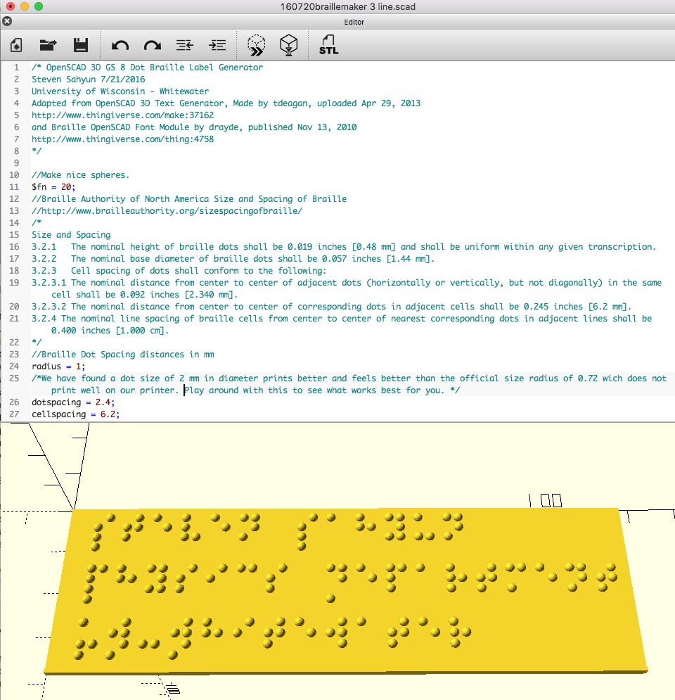
Braille Label Maker
This is the OpenSCAD file created to easily generate Grade 1 GS Braille. In the code, simply type the text you want on your label and the script does the rest. This script can be used to create labels of several rows. Note: labels with much text take a long time to render. The default braille character size is close to the Braille Authority of North America Size and Spacing of Braille at http://www.brailleauthority.org/sizespacingofbraille/ though we have found a dot size of 2 mm in diameter prints better and feels better than the official radius of 0.72 wich does not print well on our printer. Play around with this value to see what works best for you. The labels pictured above were printed with two high contrast colors filaments so that the braille text can more easily be seen. To do this, we paused the printer just before the braille layer and switched filament colors.
This code has been adapted from OpenSCAD 3D Text Generator, Made by tdeagan, uploaded Apr 29, 2013 to http://www.thingiverse.com/make:37162 and Braille OpenSCAD Font Module by Drayde, published Nov 13, 2010 to http://www.thingiverse.com/thing:4758
File to download:
 Braille Label Maker OpenSCAD script .scad
Converging Lens Ray Diagrams
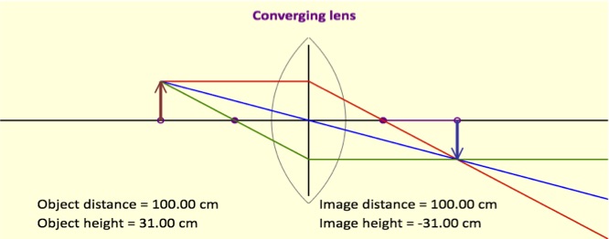
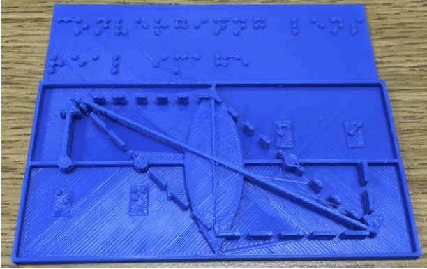
These are several ray diagrams for a converging lens for when an object is placed at half, one and a half, two times and three times the focal length of the lens. These objects have braille labeling describing the converging lens.
Files to download:
zip file of Set of four converging lens .stl files.
-
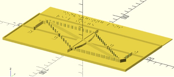 Converging Lens .scad zip file. Keep both files in the same directory when using these in OpenSCAD. OpenSCAD script created by Christopher Marshall.
OpenSCAD Converging Lens Maker file. This is the script used to generate the above files. There are two files in this zip archive, Optics_Ray_Diagram_Converging_Lens.scad and ORD_Modules.scad which needs to be placed in the same directory when running the optics ray diagram script. The ORD Modules script provides the information for creating the braille labels. In the .scad script, you can adjust the location of the object and the image and rays will be automatically calculated.
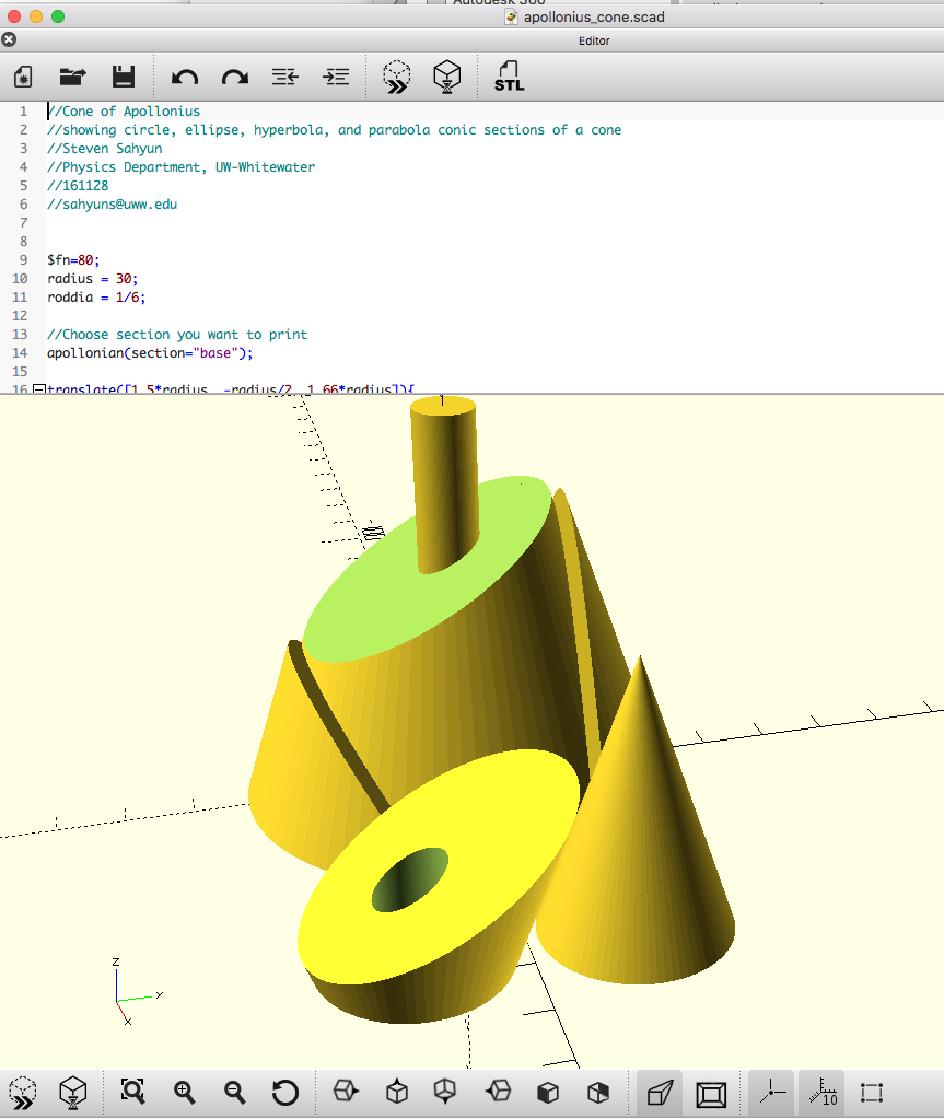
Cone of Apollonius: Conic Sections
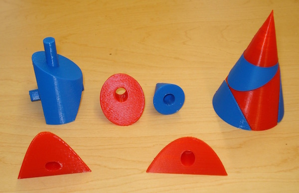
The Cone of Apollonius of Perga demonstrates the following geometrical objects that can be made from slicing a cone: circle, ellipse, parabola and hyperbola. Quadrivium.info has a nice article by Dennis and Addington about conic sections for Apollonius' cone.
This printable cone contains posts so that the parts can be conveniently assembled. The arrangment of objects when printing provides support to the posts so there is no need for additional support structures. This object was created using OpenSCAD.
File to download:
Apollonius cone .stl.zip
This model can be printed at any convenient size.-
 .zip file of Apollonius' Cone OpenSCAD script (.scad)
Standing Waves in Tubes and Strings
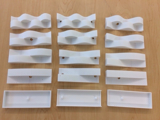
The interference of left and right propagating waves can create the phenomenon of Standing Waves. Standing waves in a finite system (such as a tube or string) have fixed (nodes) or free (antinode) endpoints.
This is a set of the first four resonant modes for three types of tubes or fixed and free end systems.
- Closed-Closed system: For a tube with two closed ends or string with two fixed end points. This model has n = 1, 2, 3, and 4
- Closed-Open system: For a tube with one end open or a string with one free end. This model has n = 1, 3, 5, and 7.
- Open-Open system: For a tube with two closed ends or string with two fixed end points. This model has n = 1, 2, 3, and 4
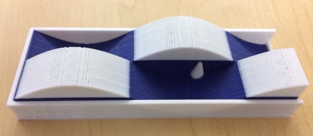
These models have boxes representing the tubes (for example: a cylindrical air column container) or the string ends. The height of the containing box represents neutral displacement (zero line) and the wave is deflected above or below (or greater air motion). The wave inserts have peg and hole arrangements specific to their type: the closed-closed column has one conical peg in the center; the open-open tube has two pegs, one on each end; and the closed open has one peg near the open end). Therefore, only the correct wave type will fit the box. The waves show two points in time: the standing wave position (displacement) at maximum displacement and half a period later.
This object was created using OpenSCAD.
File to download:
Standingwaves.stl.zip
This set of 15 models can be printed at any convenient size.
The .zip file consists of an archive of 15 .stl objects:
Three standing wave box "tubes":  closed-open and open-open:
Closed-Closed tube: StandingWavetube-cc.stl
Closed-Open tube:   StandingWavetube-co.stl
Open-Open tube:     StandingWavetube-oo.stl

There are the first four harmonic standing waves inserts for each of the tube types:

Wave inserts for Closed-Closed tube:
n=1, one-half wavelength:     StandingWave2-4cc.stl
n=2, one wavelength:          StandingWave4-4cc.stl
n=3, three-halves wavelength: StandingWave6-4cc.stl
n=4: two wavelengths:         StandingWave8-4cc.stl

Waves inserts for Closed-Open tube:
n=1, one-quarter wavelength:     StandingWave1-4co.stl
n=3, three-quarters wavelength:  StandingWave3-4co.stl
n=5, five-quarters wavelengths:  StandingWave5-4co.stl
n=7: seven-quarters wavelengths: StandingWave7-4co.stl

Wave inserts for Open-Open tube:
n=1, one-half wavelength:     StandingWave2-4oo.stl
n=2, one wavelength:          StandingWave4-4oo.stl
n=3, three-halves wavelength: StandingWave6-4oo.stl
n=4: two wavelengths:         StandingWave8-4oo.stl
Goalball Court Map
Goalball is a team sport designed for those with vision impairment. Because the goalball court is fairly large, it is helpful to have a tactile object so players learning the game can feel where the parts of the court are. This is a 3D printable map of a Goalball court with the main play areas labeled in braille. There is a small cube in the upper right corner of the object to orient the reading of the map.
This object was created using OpenSCAD.
This model has been uploaded to YouMagine as: Goalball Court Map
File to download:
goalball.stl.zip Labeled version of the goalball court.
goalball_nolabel.stl.zip version of the court without labels.
Bowling Lane Maps
These models are representations of a pair of bowling lanes. Since bowling lanes are long and are not usually able to be walked on, these models provide access to understand the relative dimensions and object locations on a bowling lane. There is usually a ball return stand located between a pair of lanes and these models show two lanes, the ball location, the foul line mark, the gutters, and the pins. Floor markings are included for partially sighted who may be able to see them on the lane. There are two models presented here: The bowlinglane_full hows the full length of the lane and ball and pin locations to scale.
The second model, bowlinglane_zoom, shows a closer view of the lanes with a zig-zag break line indicating the portion of the lanes where there are no marks or pins. To the right of the lanes, this model shows the pin locations with numbered labels. The pin diameter to placement spacing is to scale.
The models have labels indicating the approach, foul line, pins, and balls. There is a small cube in the upper right of the models to help with orientation for reading the model.
These objects were created using OpenSCAD.
These models have been uploaded to YouMagine as: Bowling lane - full and Bowling lane - zoom
File to download:
bowlinglane_full.stl.zip Full view of a bowling lane with labels.
bowlinglane_zoom.stl.zip View of the most important parts of a bowling lane with the pins labeled.
Electrostatic Potential Surfaces for + and - Charges
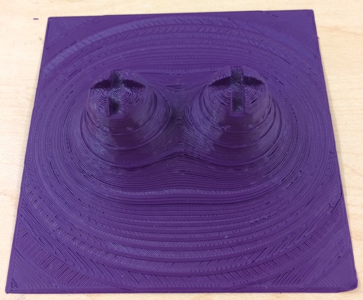
These models represent an electrostatic potential surface due to a positive and a negative charges and a surface due to two positive charges. Each surface has several equipotential lines in higher relief so it is easier to feel where the potential is equal. Recommended print size is 10 cm x 10 cm x 8 cm for the positive and negative charges, and 10 cm x 10 cm x 4 cm for the two positive charges. Print time is 2 hours each. Objects developed as a project with UW-W Student Aiden Bates.
These objects were created using a modified MATLAB script by Praveen Ranganath to create the potential surfaces and then importing the data files into OpenSCAD to add the charges and create the equipotential lines.
Files to download:
esurfaces.zip.
- MATLAB, Octave and OpenSCAD code to create esurfaces: esurface.m.zip.
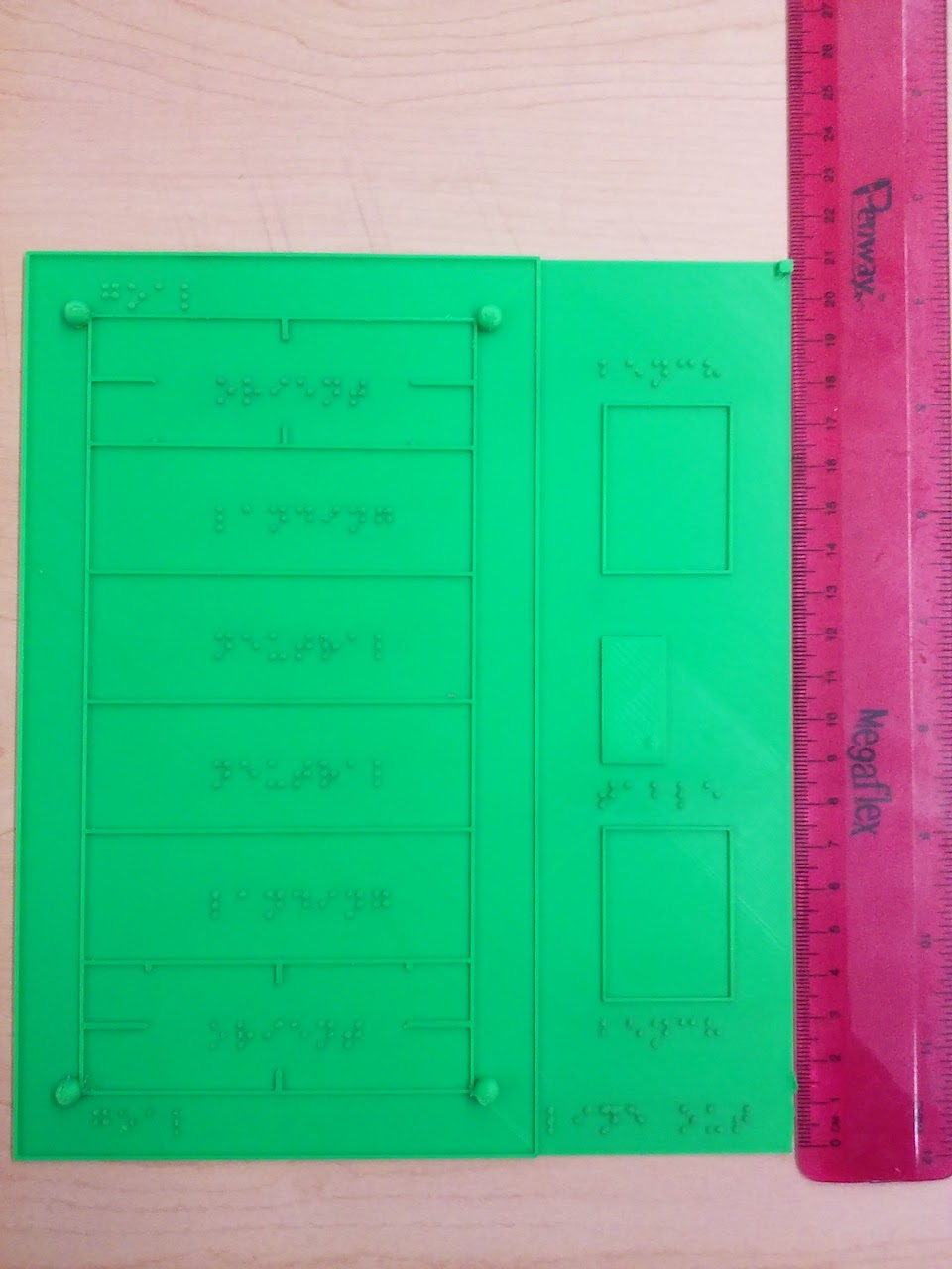
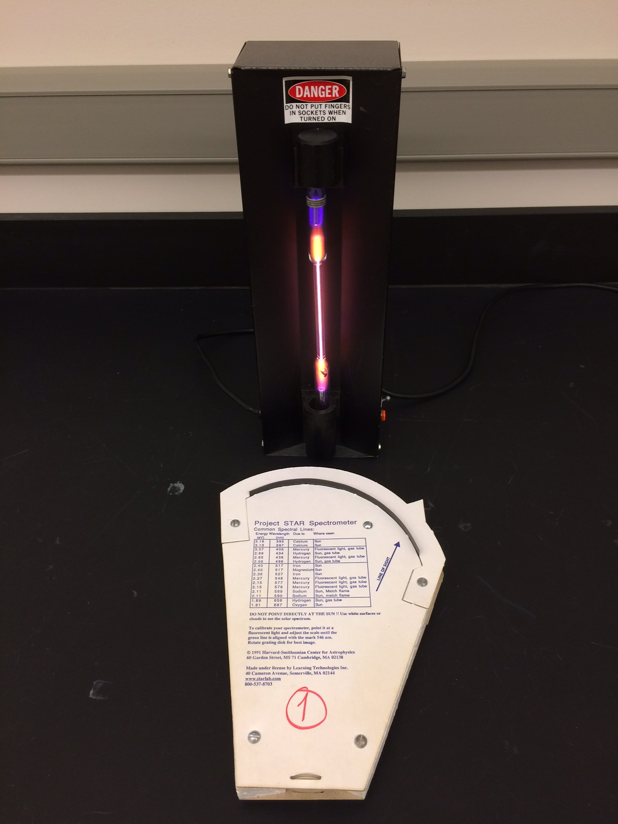
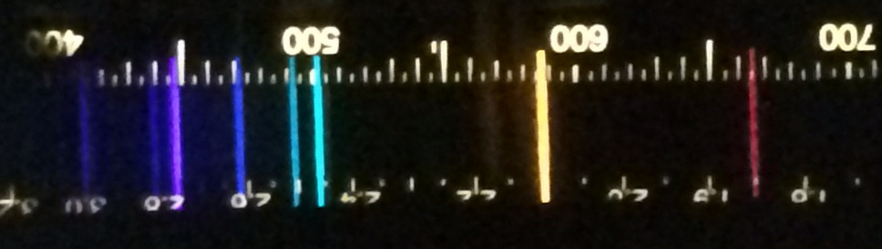
Emission Spectra of Common Elements
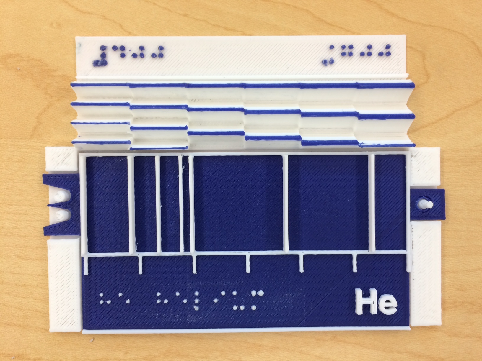
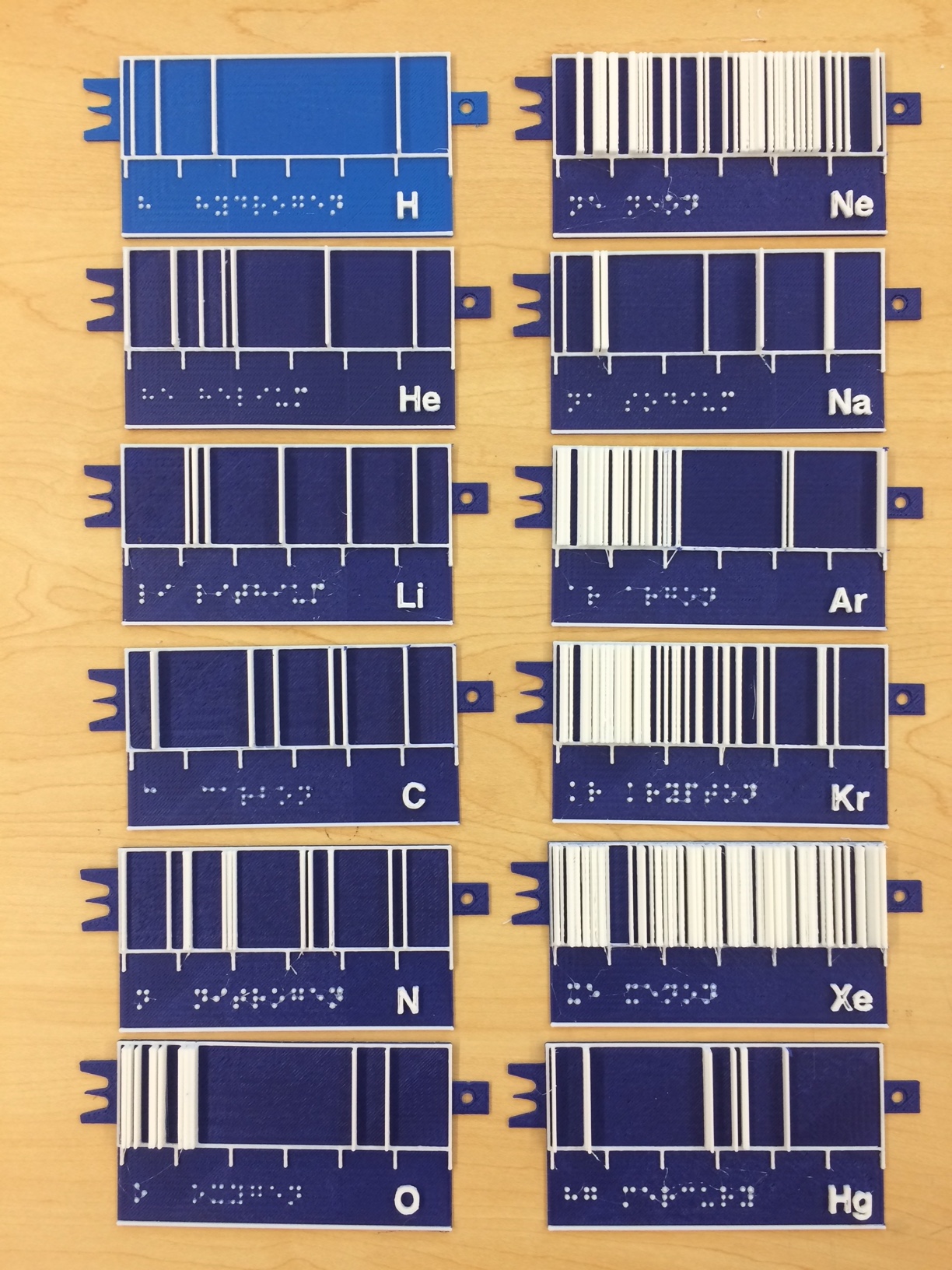
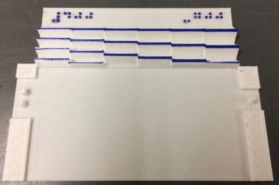
These models are the atomic emission spectra of common elements as seen using a spectrometer with a diffraction grating. The models consist of two parts, a top plate that contains the element emission lines and an optional bottom guide plate that contains a representation of the visual spectrum for reference.
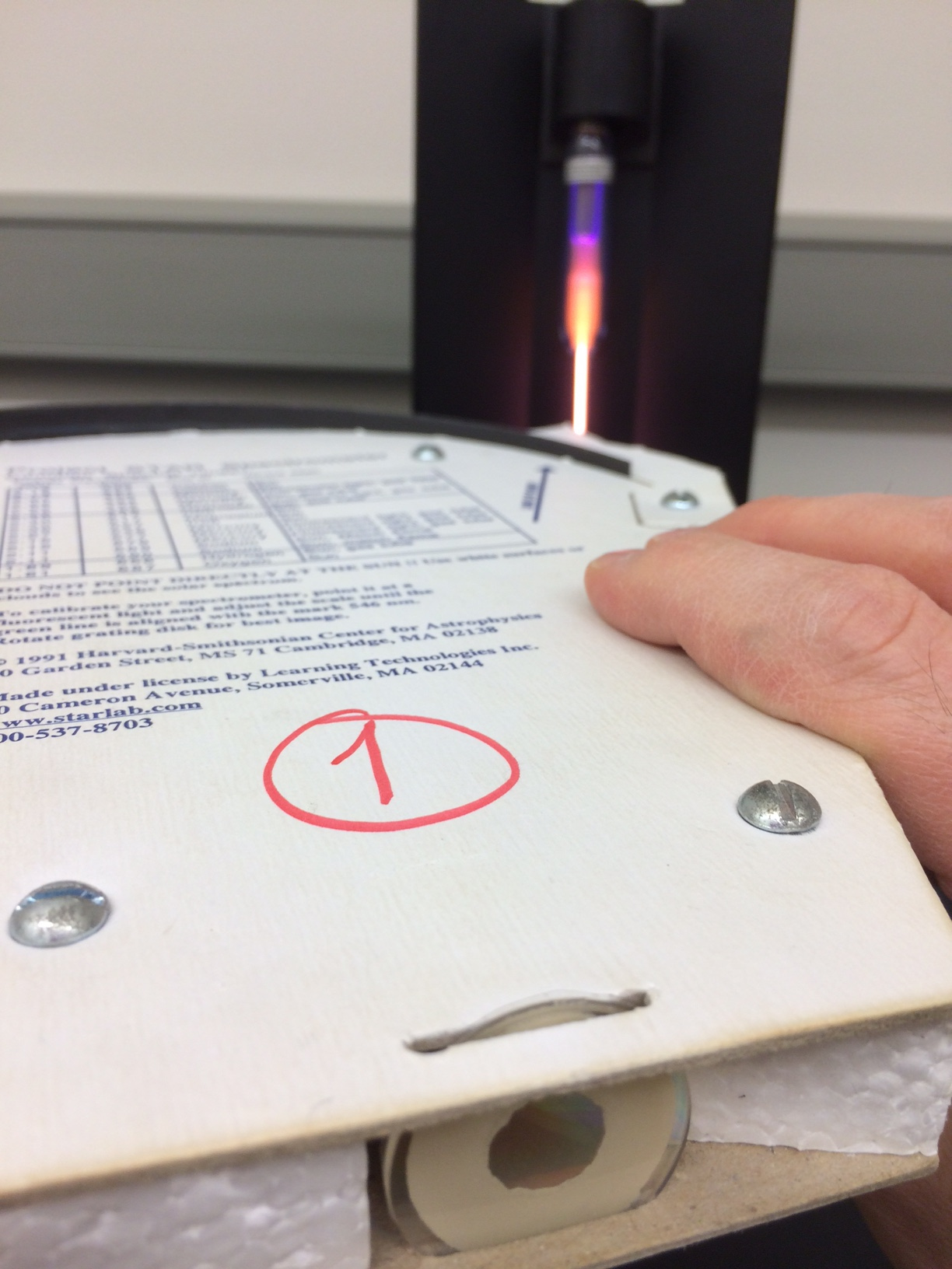
This set contains emission spectra for Argon (Ar), Carbon (C), Helium (He), Hydrogen (H), Iron (Fe), Krypton (Kr), Lithium (Li), Mercury (Hg), Neon (Ne), Nitrogen (N), Oxygen (O), Sodium (Na), and Xenon (Xe).
The elemental emission spectra start at 400 nm on the left through 700 nm on the right with height representing the observed brightness of the line. The emission wavelength and brightness were tabulated from data atNIST Atomic Spectra Database
Each element plate features the element symbol in braille, raised text, and the element name in braille. There are wavelength tick marks every 50 nm at the bottom of the plate. The plate has a three-prong tab on the left and a tab with a hole on the right side for easy insertion to the base plate.
The bottom spectrum guide plate guide has wave patterns representing 400, 450, 500, 550, 600, and 650 nm light waves so students can feel where on the spectrum an emission line resides. It is marked in braille with 400 in the upper left and 700 in the upper right. The left side has two posts for the three-prong element tab and the right has a cone post to easily place the element plate's right tab hole.
These objects were created using OpenSCAD.
These models have been uploaded to YouMagine as: ... test
File to download:
The first file is the set suitable for printing with a single filament 3D printer. This second file has the lines, and lettering as a separate file for use with dual-filament 3D printers. To print select the bottom file and insert the element of your choice. Set the color for one of the files and then click align. It should be ready to print then. Dual-Color models made with assistance from UWW Student Joel Heaberlin.Scale Model of the Solar System
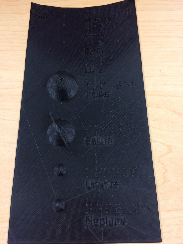
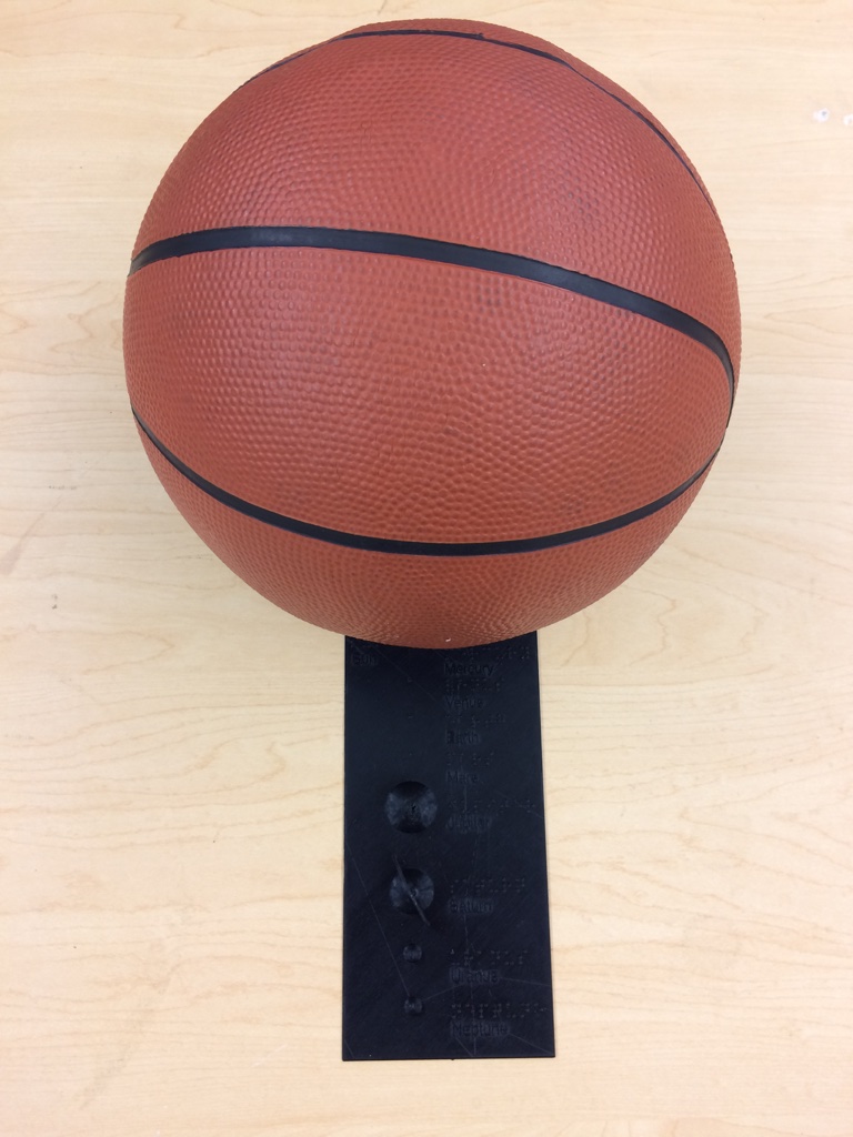
This is a scale model of the sizes of the eight planets in the solar system. In this model, there is a cutout to represent the Sun. The scale of the model is such that the Sun may be represented with a basketball, and can be placed in the cutout area. There is a square locator for the upper right of the object for proper reading orientation. The planets are labeled in braille and text.
These objects were created using OpenSCAD.
File to download:
Scale Model for Solar Eclipse
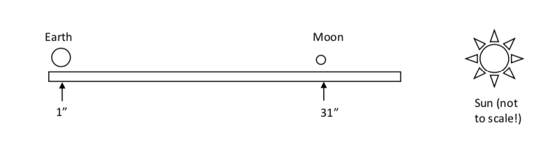
This model shows the scale of the Earth and Moon. The object attach to a standard meter stick. Place the Earth at 1-inch and the Moon at 31-inches. In this model, the Earth is a 1-inch sphere and the Moon is located at 30 times the Earth's diameter.
In this model, Earth is represented by the larger 1-inch ball and the Moon is represented by the smaller 1/4-inch ball. The Moon orbits 30 Earth diameters away, so on this scale, Earth is placed at the 1” mark of a yardstick and the Moon is placed at the 31” mark. Placing the Moon between the Earth and the Sun (light source) will cast a shadow of the Moon onto the Earth and you can produce your own mini-eclipse!
When oriented with the Moon towards the Sun, the Moon's shadow will fall on the Earth.
These objects were created using OpenSCAD.
File to download:
Inverse Square Law
 Image Source: Wikipedia: Inverse Square Law. |

|
This model shows the relationship of uniformly spreading energy with distance from a point source as discussed in the Hyperphysics page on the inverse square law and the Wikipedia page on the Inverse Square Law. The model has tactile indicators representing each unit area and contains text and Braille labels for 1r, 2r and 3r. It also has an orientation block in the upper right corner of the model.
This object was created by Ian Cooper and Steven Sahyun, 2024
File to download:
inversesquarelaw.stl.zip.
This .zip file contains the .stl model to print directly.inversesquarelaw.zip.
This .zip file contains two OpenSCAD source files: inversesquarelaw.scad and brailletext.scad which the first imports to display the Braille characters.
Source Files:
test


These models ... test test
These objects were created using OpenSCAD.
These models have been uploaded to YouMagine as: ... test