-
9.
- Overview
- Sample
This experiment was the culmination of the techniques used in the pilot tests. While the Web pilot test formed the basis and instrumentation for this experiment, there were some major modifications to the main test questions. The main test questions were rewritten to produce better data for analysis. The number of questions expanded to include questions concerning mathematical functions, as well as questions to probe physics concepts. The Web pilot also noted the need for improved introductory material. This was also implemented in the Main Auditory Graph test.
The original goal of the auditory graphing method was to provide visually disabled people with a method for quickly accessing information that was otherwise portrayed by a visual modality. The Main Auditory Graph test therefore included a small group of blind subject volunteers to evaluate the effectiveness of these graphs with the intended user. This group of subjects was not used in the pilot tests due to the extreme scarcity of subjects fitting the testing requirements.
The subject population was enlarged to include undergraduate students from several institutions, as well as graduate students to check the reliability of test questions, and blind volunteers.
9.As the testing process was designed for first year physics students, instructors of these courses at several educational institutions were solicited during the Spring and Fall 1998 terms for the possibility of letting their students participate in this study. It was arranged with one instructor at Oregon State University (OSU) and one instructor at Pacific University (PU) of introductory, algebra based, physics courses to provide extra credit homework points to students taking Web pilot test. An instructor of a calculus based introductory course at Pacific University also had her students participate for credit.
An instructor of an algebra based physics course at Linn-Benton Community College (LBCC), and a professor of a calculus based course at OSU mentioned the study and web address in class but did not offer credit for participation.
OSU Graduate student subjects were informally solicited throughout 1998 for their help to test the reliability of the questions and auditory method. These subjects took the test with the auditory graph presentation method. There are four graduate subjects scores that are not reported. Two were due to technical difficulties that the subjects had when taking the test while the other two used the wrong class code and received a test with visual graphs.
Student subject participation from each physics course was not uniform. There were two factors for this. The most important factor for participation was the willingness of the instructor to issue extra credit for participation. While the received credit such that it virtually played no part in the overall grade that the student received, participation from these courses was generally over 50%. When extra credit was not given, participation was greatly reduced. The second most important factor was course size. However, credit was by far the dominant factor.
Blind subject volunteers who had experience with college level physics and who where willing to participate in a web based test were solicited by posts to e-mail lists, and through personal contact at conferences. Interested subjects were sent informational packets containing tactile graphs, introductory information, and the web address location in a braille format. A computer diskette containing the same text as the braille information was also included in the packet. Blind subjects participated throughout 1998.
There were five blind subjects who participated as subjects, and one who was consulted for development and acted as a critical evaluator of this study. Although this is a fairly small number, this level of participation is a significant achievement as none of the test subjects participated locally. One of the subjects participated internationally from Europe, the other four were domestic. From solicitations, there were 15 interested volunteers who provided a mailing address for the information packets. Of this number, six subjects decided to participate and were able to access the web page test. One participant was unable to complete the test due to technical difficulties.
The following table shows the distribution of the subjects with regards to the course, school and approximate course size from which they were drawn.
Table .1 Distribution of Subjects per Course
|
Course |
# subjects |
Approx. Course Total |
Date |
|
OSU 203, algebra |
186 |
350 |
Spring 98 |
|
OSU 213, calculus |
2 |
200 |
Spring 98 |
|
LBCC 203 |
4 |
20 |
Spring 98 |
|
PU, algebra |
28 |
44 |
Fall 98 |
|
PU, calculus |
8 |
30 |
Fall 98 |
|
Graduate |
6 |
N/A |
98 |
|
Blind |
5 |
N/A |
98 |
Of the 186 subjects in the OSU 203 course, 85 had taken the Web pilot test. Subjects from physics classes were randomly assigned to one of three test groupings. Of the 231 subjects, 74 subjects received auditory graph, 76 received visual graph, and 81 received both auditory and visual graph presentation methods. These numbers allow for statistically significant results at the p = 0.05 level since for three test groups, the number of subjects in each group should be greater than 62 (from Equation 3.2).
9.Data was collected in a similar manner as for the Web Pilot test. After an initial welcoming and informed consent page, all subjects were given a short tutorial on the auditory graph presentation method with several examples for them to try. The tutorial consisted of a series graph descriptions, images and sound files of increasingly complex auditory graphs for them to experience. After the introductory page, there was a log-in page to record the subject's name and class code. PERL script programs recorded subjects' answers and presented them with subsequent web question pages in an identical fashion to the Web Pilot test. Material pertaining to the Main Auditory Graph test can be found in Appendix F.
At the end of the test, the subjects were presented with a page that thanked them for their participation, and contained links to a page of correct answers, an e-mail response form for any comments, informational pages on how the graphs were developed, as well as a link to the Science Access Project home page.
9.The survey and pretest were identical to those of the Web Pilot. The main test section however had been considerable altered from the pilot studies. To better determine how well subjects were able to identify graphs, versus how well they can use those graphs for interpretation of physical phenomena, the main test was divided into two sections, math and physics, of 17 questions each. The virtually identical graphs were repeated in the same order between the math and physics sections, although there was one graph which was different between the sections. This graph consisted of point discontinuities in the math section, but the corresponding graph in the physics section was that of a black body spectrum. The rationale for having two sections of similar graphs was so that split-half analysis of the sections could be performed to investigate consistency and performance issues relating to identification or analysis type questions.
The first question in each section consisted of a linear graph with 0 slope. Aside from this graph, there were 8 pairings of similar graph types. Thus, each graph type would appear twice in each section of the test. Graphs were grouped in the following categories: linear, step function, simple positive curvature, simple negative curvature, linear and curved composite, simple curved peak, complicated functions, and multiple peaked. The rationale for having two graphs of each group was to allow for a split-half analysis of each subject test.
As this was a somewhat iterative process, questions were developed based on the graphs, and graphs were chosen based on the types of questions that could be asked of them. Several, but not all of the questions from the pilot test were utilized for this test. Questions were also chosen based on a diverse range of physical phenomena and their prevalence in the subject matter of introductory math and physics courses. The graphs and questions were reviewed by several Math, Physics, and Science Education faculty for content validity. The graphs and corresponding questions can be found in Appendix C.
There were a few modifications to the display of the graphs on the web pages. As these auditory graphs had no method to label their axes, the range of data values was explicitly stated in the questions. Also, several subjects in the Web pilot test noted that it was difficult to tell where the zero point on the auditory graphs were. For this reason, a link to a MIDI file playing the pitch of the zero representation was included with the graph with the idea that subjects could compare the "zero" pitch to the pitch on the graphs. The zero sound for all graphs was identical. After this test, a couple subjects commented via e-mail that this was not particularly helpful.
Other changes to the test included providing more complete annotation of images by the use of the "alt" tag field for images. All images were labeled in this manner. Equations that were displayed in the test were done so by displaying small graphic images of the equations. The images were produced with Microsoft Excel 5. All equation images were alt tagged with a linear notation for the mathematics.
The entire test was checked for compatibility with the JAWS screen reader and Internet Explorer. As noted in the Web pilot, the auditory graph sound files were displayed in three formats so that users could pick the format that was most compatible with their system. The test was also checked for coherent keyboard access to all links and text entry fields.
These last issues were vitally necessary for the blind subjects to be able to access, take, and understand the test.
The introductory material and pre-test contained visually presented graphs. Blind subjects had been sent information packets containing these graphs represented in a tactile format as a high resolution graphic image produce by the TIGER printer at OSU. Unfortunately, the informational packets were often ignored and the pretest questions went unanswered by a majority of the blind volunteers.
9.The following table is a summary of more complete results contained in Appendix C. The table is divided by results from the different test groups for the pre-test and math and physics sections of the main test. Labeling for groups is as follows: S for the group with auditory graphs (sound), V for visually presented graphs, B for both auditory and visual graphs, G for graduate student subjects, and N for blind subjects (non-sighted.)
Table .2 Table of percentage of correct answers per group for each problem.
|
Question |
V - Visual |
B - Both |
S - Sound |
G - Grad |
N - Blind |
|
Pre-Test |
|||||
|
p1 |
72% |
83% |
78% |
100% |
20% |
|
p2 |
95% |
96% |
97% |
83% |
20% |
|
p3 |
93% |
89% |
93% |
83% |
20% |
|
p4 |
67% |
81% |
89% |
100% |
20% |
|
p5 |
55% |
68% |
66% |
100% |
20% |
|
Main Test |
|||||
|
Math Section |
|||||
|
m1 |
84% |
64% |
57% |
100% |
100% |
|
m2 |
86% |
79% |
46% |
83% |
100% |
|
m3 |
82% |
80% |
77% |
100% |
100% |
|
m4 |
78% |
79% |
76% |
100% |
100% |
|
m5 |
80% |
83% |
69% |
100% |
100% |
|
m6 |
61% |
42% |
24% |
67% |
80% |
|
m7 |
83% |
81% |
70% |
100% |
100% |
|
m8 |
76% |
78% |
68% |
100% |
80% |
|
m9 |
66% |
68% |
45% |
100% |
60% |
|
m10 |
62% |
75% |
55% |
83% |
80% |
|
m11 |
58% |
58% |
36% |
100% |
80% |
|
m12 |
38% |
38% |
14% |
67% |
40% |
|
m13 |
68% |
65% |
49% |
83% |
80% |
|
m14 |
28% |
17% |
22% |
83% |
40% |
|
m15 |
66% |
63% |
59% |
83% |
80% |
|
m16 |
49% |
46% |
46% |
100% |
80% |
|
m17 |
30% |
26% |
28% |
100% |
80% |
|
Physics Section |
|||||
|
m18 |
57% |
51% |
41% |
83% |
100% |
|
m19 |
42% |
35% |
35% |
33% |
60% |
|
m20 |
21% |
28% |
19% |
83% |
80% |
|
m21 |
41% |
41% |
26% |
83% |
20% |
|
m22 |
76% |
81% |
84% |
100% |
100% |
|
m23 |
62% |
44% |
58% |
50% |
80% |
|
m24 |
72% |
79% |
62% |
100% |
100% |
|
m25 |
70% |
62% |
49% |
100% |
100% |
|
m26 |
58% |
62% |
36% |
100% |
60% |
|
m27 |
63% |
64% |
50% |
100% |
100% |
|
m28 |
54% |
58% |
27% |
100% |
100% |
|
m29 |
54% |
43% |
35% |
83% |
40% |
|
m30 |
45% |
48% |
54% |
17% |
80% |
|
m31 |
37% |
36% |
42% |
83% |
60% |
|
m32 |
72% |
70% |
62% |
100% |
80% |
|
m33 |
72% |
70% |
64% |
100% |
100% |
|
m34 |
18% |
16% |
23% |
17% |
0% |
For the V, B, and S groups, equation 2.2 yields a maximum value of:
![]() . This result is the 95%
probability that the average values for each question are correct to
within a 4 percentage point error limit. For example, there is a 95%
certainty that the Main test question number 33 for the Both group is
between 60% and 68%.
. This result is the 95%
probability that the average values for each question are correct to
within a 4 percentage point error limit. For example, there is a 95%
certainty that the Main test question number 33 for the Both group is
between 60% and 68%.
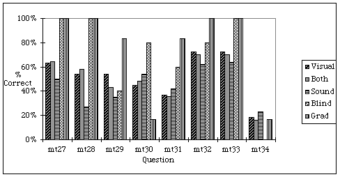
While the summary table provides an accurate listing of the data, it is helpful to view the same data as a bar chart to recognize patterns in the data and to easily see where any difficulties may lie. For example it can be easily seen that question 34 has an unusually low result. It shows the effect of a poor question as all groups performed at the level of random guessing.
The following charts display the percent correct scores for each testing group vs. the individual test questions. The charts are divided by test section.
Figure .1 Pre-test: Avg. % Correct per Group.
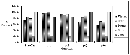
Figure .2 Math Section: Avg. % Correct per Group. Questions 1-9
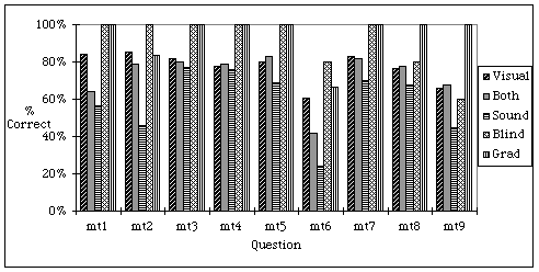
Figure .3 Math Section: Avg. % Correct per Group. Questions 10-17
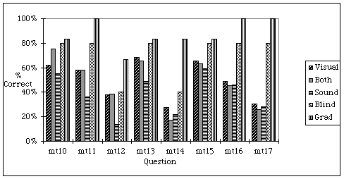
Figure .4 Physics Section: Avg. % Correct per Group. Questions 18-26
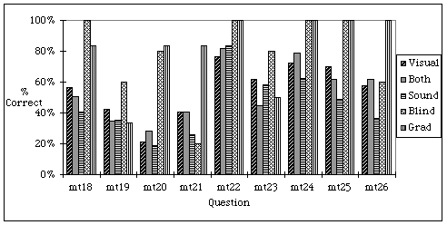
Figure .5 Physics Section: Avg. % Correct for Questions 27-34
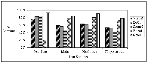
Average values for the test sections, and standard deviations of the averages are given in the following table.
Table .3 Average % Correct per Section Per Group
|
Group: |
Both |
Sound |
Visual |
Grad |
Blind |
|
Average, Pretest |
83% |
85% |
77% |
93% |
20% |
|
Standard deviation (s ) |
10% |
13% |
17% |
9% |
0% |
|
Average, Main |
57% |
47% |
59% |
85% |
78% |
|
s |
20% |
18% |
19% |
23% |
25% |
|
Average, Math Section |
61% |
49% |
64% |
91% |
81% |
|
s |
21% |
20% |
19% |
12% |
19% |
|
Average, Physics Section |
52% |
45% |
54% |
78% |
74% |
|
s |
18% |
17% |
18% |
30% |
31% |
|
Average time to Complete |
30 min. |
34 min. |
24 min. |
40 min. |
41 hrs. |
Note: The average pretest score for the Blind group reflects the result that only one blind subject completed the pretest. That subject answered all pretest questions correctly. The large average time value for the Blind group was due to several of the subjects starting part of the test, and returning a day or two later to complete the test as their schedule permitted. The average time for the two blind subjects completing the test in one day was 79 minutes.
Figure .6 Summary: Avg. % Correct per Group for Each Section
-
9.6.
- Reliability
Examination of the percent correct scores for the different groups can lead to some indication of the reliability of students to successfully answer the questions. Graduate student subjects were solicited as subjects with a large amount of experience with the physics material and graphs. The received the test with auditory graphs to determine what would be the best expected results on the auditory graph. If the graduate students consistently missed specific questions, then careful examination as to their validity is necessary.
Two graduate subjects inadvertently received the visual test. These subjects each missed one question (number 8 for one, and number 30 for the other,) so these questions are of concern. More importantly are the questions where a majority of graduate students using the auditory graphs gave incorrect answers. This occurred for three questions 19, 30, and 34.
Question 19 involved a linearly increasing graph, representing velocity vs. time. The most common answer (3 of 6) was " D: The object is moving with a constant velocity," whereas the correct response " The object is moving with a constant, non-zero acceleration." was only answered by two subjects. It is suspected that the subjects were not paying close attention to the statement describing the axes values and representation. Given that all other groups (including the S group) outperformed the graduate students on this question, and that the two graduate subjects both answered this question correctly, the question was retained as valid.
Question 30 involved the identification of an intensity pattern produced
by a double slit source. Five of six graduate students (and one of the
visual test grads) identified the pattern as that of a single slit source.
While there are similarities between the two patterns, the other subjects
groups correctly identified the pattern at a minimum of the 45% level. Due
to the good response rate from the other groups, this question was
retained.
Question 34 involved a determination the initial conditions for the motion of a mass suspended by springs on a cart. Several of the graduate students mentioned that the question was confusing and responses from all groups followed a random distribution between possible answers. Thus, question 34 was a poorly designed question, and was dropped from the analyses.
Recalculating the average correct scores for the Main and Physics sub-test without question 34 adjusts the Main and Physics sub-test averages.
Table .4 Recalculation of % Correct without #33
|
Both |
Sound |
Visual |
Grad |
Blind |
|
|
Main |
58% |
48% |
60% |
87% |
80% |
|
Physics sub-test |
55% |
46% |
56% |
82% |
79% |
In split-half analysis, the correlation value r is a measurement of how well the results of one sub-test correspond to theoretically equivalent questions in the second sub-test. An r = 1 value indicates perfect correlation, and the two tests are identical. A value of r = -1 indicates that a subject who answering correctly on one sub-test, answered the split question incorrectly and vice versa. An r = 0 value indicates no correlation between the two sub-tests.
As noted in the section on Instrument Design, the main test had two sub-tests, Math and Physics, containing similar graphs. Each of these sub-tests were designed to be divided into two tests containing graphs of similar nature such as derivative and complexity. For example a graph of y = x was paired with a graph of y = A - x, and y = x2 was paired with y = 1/x.
Table 9.5 lists the split-half correlation values between and within the Math and Physics sub-tests for each of the groups (B - Both, V - Visual, and S — Sound.) The Blind (N), and Grad (G) groups are included for completeness, but it should be stressed that due to the small nature of these last two groups, the results may not be valid. Since question 34 was found to be unreliable, it and it's split question (17 in the between Math/Physics split, and 30 in the within Physics split) were removed for calculations of the correlation coefficients.
Table .5 Correlation r for Groups
|
Test |
B |
V |
S |
N |
G |
|
Main |
0.28 |
0.04 |
0.09 |
0.33 |
0.49 |
|
Test A Math questions 1-16 |
|||||
|
Test B Physics questions 18-33 |
|||||
|
Math |
0.55 |
0.67 |
0.31 |
0.87 |
0.09 |
|
Test A: 2,4,6,7,9,12,13,15 |
|||||
|
Test B: 3,5,8,10,11,14,16,17 |
|||||
|
Physics |
0.31 |
0.16 |
0.01 |
0.38 |
0.17 |
|
Test A: 19,21,23,24,26,29,32 |
|||||
|
Test B: 20,22,25,27,28,31,33 |
While there is moderate correlation between the sections in the Math sub-test, there is only very poor correlation between the sections of the Physics sub-test. Also, there is very poor correlation between the Math and Physics tests.
The conclusion of the split half analysis is that the Math sub-test was moderately successful in creating two equivalent tests. However, it should also be noted that the Sound group did not share the same level of correlation between the two Math sub-tests, in fact they only have a poor correlation value. The performance of auditory graphs in the Math section appears to produce some added inconsistencies in the test results.
The Physics sub-test did not produce correlated results between its sections. This is perhaps related to a poor choice of questions. A more likely explanation is that in these questions, subjects were answering questions about physical phenomena, and this was a more significant effect than the graph type. As the nature of the physics in the questions was different for each questions, student understanding and performance ability varied, irrespective of the displayed graph.
Thus, for the math questions, there was greater reproducibility in the scores with regards to graph type than was seen with the physics questions. The difference in performance may be due to the math questions being more of a descriptive choice, whereas the physics questions involved more interpretation and understanding of physics. If the physics is not well understood, this could play a significant effect on ability to interpret the graph.
9.6.All of the t-tests performed were calculated with Microsoft Excel. The t-tests were all calculated as two sample assuming unequal variances with \alpha = 0.05 and a hypothesized mean difference of 0. All tcritical values were chosen to be two-tailed. ANOVA calculation were single factor with a = 0.05. In other words, the results of the tests have a 95% confidence limit.
ANOVA and t-test scores are given first for the S, B, and V groups. It should be kept in mind that these three groups have more statistical relevance as the sample sizes from which the means were calculated were between 74 and 81. The G and N groups had sample sizes of 6 and 5 subjects on which to calculate the means values.
The first question to ask is "Are the differences in the average percent correct scores between the S, B, and V groups on the Pre-test significant?" ANOVA comparing S, B, and V groups yielded the result of F = 0.52, and F Critical = 3.88. F is a value that compares the correlated variances in paired samples. Since F < F Critical, there was no significant difference between the three groups. Thus, the performance levels of the subjects was randomly distributed between the groups.
A judgment on the significance of the differences between the average percent correct scores of the S, B, and V groups on the Main test can also be provided by ANOVA. The result of F = 3.73, and Fcritical = 3.09 indicates that there were significant difference between the groups since F > Fcritical.
To determine where the significant difference exist, a set of
pre-planned pair-wise t-tests was performed. The calculated t is the
deviation of the sample mean from the population mean, measured in units
of the mean's standard error,![]() ,
where s
is the standard deviation, and n is the number of samples. [Sne89, p. 44]
It is a test of equivalence between two groups. The value of
tcritical is a calculated value such that there is a 5%
probability that the value will be exceeded t. If the calculated t <
tcritical then there is no significant difference between the
pairs.
,
where s
is the standard deviation, and n is the number of samples. [Sne89, p. 44]
It is a test of equivalence between two groups. The value of
tcritical is a calculated value such that there is a 5%
probability that the value will be exceeded t. If the calculated t <
tcritical then there is no significant difference between the
pairs.
A series of pre-planned t-tests comparing the results of the S, B, and V groups for the test as a whole, and for the Math and Physics sections separately are given in Table 9.6. There is also an indication of whether or not a significant difference between the groups exists. Tcritical is based on a two-tailed test.
As a matter of convention, differences between groups will be calculated as the subtraction of the percent correct of one group from that of a second group. For example, the average percent correct on the Main tests (questions 1 through 33) for the Visual group was 60%. The average percent correct for the Sound group was 48%. The difference in the scores is thus 12%.
Table .6 T-tests Between Groups.
|
Group pair |
T |
tcritical |
Difference |
Significant |
|
|
S-V |
Main |
-2.8 |
2 |
12% |
Yes |
|
Math |
-2.27 |
2.04 |
15% |
Yes |
|
|
Physics |
-1.65 |
2.04 |
10% |
No |
|
|
S-B |
Main |
2.22 |
2 |
10% |
Yes |
|
Math |
1.73 |
2.04 |
12% |
No |
|
|
Physics |
1.37 |
2.04 |
9% |
No |
|
|
B-V |
Main |
-0.48 |
2 |
2% |
No |
|
Math |
-0.44 |
2.04 |
5% |
No |
|
|
Physics |
-0.26 |
2.04 |
1% |
No |
Thus, t-tests reveal that there is a significant difference between the Sound and Visual graph groups. This difference arises primarily from the Math test section. The Sound and Both groups have a significant difference for the whole test, but there is not a significant difference in either of the Math or Physics sub sections.
The Sound group can be adjusted so that the Pre-test results are equivalent with the Visual group by means of a weighted means. [Sne89, p. 226] This was accomplished by multiplying all of the question averages by the ratio of the average pretest scores,
![]() (9.1)
(9.1)
A t-test was then performed on the resulting adjusted scores for the S'-V physics sub-test. Results give t = 2.57 > tcritical = 2.04. Thus, there is now a significant difference for this pairing. Similarly creating a weighted value for a comparison to the Both group is given by,
![]() (9.2)
(9.2)
A t-test was then performed on the resulting adjusted scores for the S''-B physics sub-test. Results give t = 1.57 < tcritical = 2.04. The t-test for S''-B math sub-test give t = 1.86 < tcritical = 2.04. The differences between these groupings are still not significant. There was a significant difference for the test taken as a whole as noted above.
A t-test comparison between Grad (G) and Blind (N) groups showed that the 7% difference in the results was not significant (t = 0.97 < tcritical = 1.99.) This result should be viewed with caution however as the subject sample size was very small for each of these groups. (n = 6). Equation 2.2 gives a estimate that the average for each question is correct to ± 18%, so a significant result may be masked by this uncertainty.
9.6.An interesting effect was noticed when comparing average scores on the main test between subjects who were in the Sound group with musical training (47 subjects), such as learning an instrument, to those in the same group but without any musical training (27 subjects). Subjects with some music background had an average score of 16.9 of 34, whereas those without music had a score of 14.6. Measurement error for each question is calculated to be less than 7%. F test results give F = 0.90 and Fcritical = 0.57 at the a = 0.05 level. Since F > Fcritical,, there is a significant difference between groups. A two tailed t-test at the a = 0.05 level also shows that t > tcritical. When t > tcritical, the null hypothesis of the two groups being equal is retained. Thus, music training seems to have a small, but significant effect on performance levels for the auditory graphs.
9.6.The Main Auditory Graph test showed a similar difference as the Web pilot between the average times taken by the Sound and Both groups for completing the test. The time difference for the whole test was about 4 minutes, or 7 seconds per question. This is about the length of time required to listen to the auditory graph once. Thus the Both group either did not listen to the sound graphs, or the Sound group played their graphs an additional time. The time difference between the Grad and Sound groups was 6 minutes, or about 10 seconds per question. Thus the graduate students may have listened to the sound graphs a additional time or given more consideration to the questions.
9.6.